Abstract
The past decade has yielded more biodiversity observations from community science than the past century of traditional scientific collection. This rapid influx of data is promising for overcoming critical biodiversity data shortfalls, but we also have vast untapped resources held in undigitized natural history collections. Yet, the ability of these undigitized collections to fill data gaps, especially compared against the constant accumulation of community science data, remains unclear. Here, we compare how well community science (iNaturalist) observations and digitized herbarium specimens represent the diversity, distributions, and modeling needs of vascular plants in Canada. We find that, despite having only a third as many records, herbarium specimens capture more taxonomic, phylogenetic, and functional diversity and more efficiently capture species’ environmental niches. As such, the digitization of Canada’s 7.3M remaining specimens has the potential to more than quintuple our ability to model biodiversity. In contrast, it would require over 27M more iNaturalist observations to produce similar benefits. Our findings indicate that digitizing Earth’s remaining herbarium specimens is likely an efficient, feasible, and potentially critical investment when it comes to improving our ability to predict and protect biodiversity into the future.
Introduction
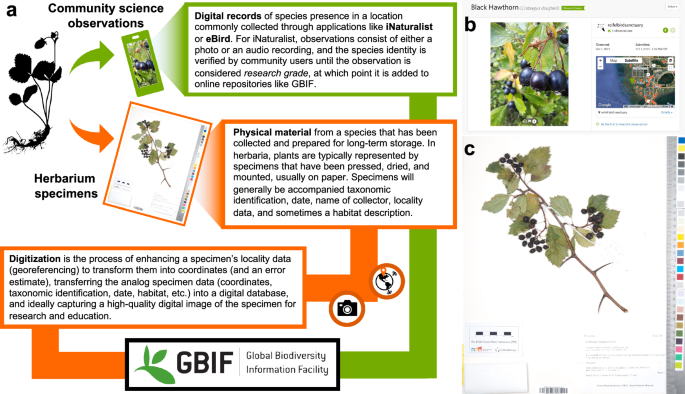
What was once the purview of trained scientists, collecting biodiversity data is rapidly becoming an endeavor of community (citizen) scientists logging species sightings into their phones rather than collecting physical specimens (Fig. 1). The Global Biodiversity Information Facility (GBIF) now has over 2.3 billion occurrence records, 50% of which were collected by community scientists since 20101. But despite this data windfall, existing information on biodiversity remains biased and largely incomplete2, limiting our ability to consider all aspects of biodiversity in conservation planning3. Overcoming these critical data shortfalls will rely on obtaining additional biodiversity data that captures the diversity and distribution of life on Earth. To that end, the digitization of Earth’s remaining natural history collections is a potentially feasible and efficient option.

Definitions (a) and examples (b, c) of community science observations, herbarium specimens, and the digitization process.
Natural history collections like herbaria might be less prone to some of the biases that pervade community science observations. While community science platforms like iNaturalist favor common and larger species and urban areas4,5, herbarium collections, despite sharing some biases6,7, better represent rare species and rural areas8 and contain a wealth of irreplaceable data9. For example, recent work by Daru & Rodriguez showed that natural history collections like herbaria outperform community science records in terms of spatial and taxonomic bias and better match expected biodiversity patterns8. However, the sheer rate at which we are accumulating community science observations may eventually negate its biases and so it remains unclear whether the digitization of Earth’s remaining 314M herbarium specimens is needed to overcome existing data shortfalls10,11.
Alongside data coverage, it is also important to understand whether we have enough data to build reliable models, which are often essential for converting biodiversity data into a form useable for conservation needs. The recent Kunming-Montreal Global Biodiversity Framework reinvigorated humanity’s effort to protect Earth’s biodiversity over the next few decades12, but to inform conservation policy amid climate change, nations around the world need a basic understanding of current and future species distributions13,14,15. Species distribution models (SDMs), which predict species occurrence across geographic space and time based on abiotic and biotic predictors, are increasingly used for this purpose. But SDM performance is limited by incomplete and biased biodiversity data that poorly capture the full extent of species’ environmental niches16,17,18. The ability of herbarium specimens versus community science observations to represent species’ niches is untested and so it remains unclear how the accumulation of additional iNaturalist observations versus the digitization of existing herbarium specimens might improve our ability to describe, quantify, and model biodiversity. To fill this gap, we assess the ability of both data types to capture the taxonomic, phylogenetic, and functional diversity and environmental niches of Canada’s vascular plants. Additionally, we leverage the coordinated network of herbaria and detailed information on the extent of undigitized herbarium collections in Canada to predict the potential gains in biodiversity knowledge and ability to model species distributions that could be accrue from digitizing remaining specimens.
We report that, compared to iNaturalist observations, herbarium records exhibit less bias and more efficiently represent both the diversity and distributions of Canadian plants. Moving forward, we estimate that the digitization of Canada’s remaining herbarium specimens could greatly benefit our knowledge of plant biodiversity, potentially quintupling our ability to model species’ spatial distributions. Finally, despite the growing rate at which we are accumulating new observations, it is unlikely that community science alone can match the benefits of herbarium digitization in the near future, pointing to the likely critical importance of herbaria and their collections for informing conservation planning to reach our 2030 goals and beyond.
Results
For all of Canada’s 4392 vascular plant species, we downloaded observation data from GBIF for Canada and the United States from the year 1900 to present (January 2024), which resulted in a total of 12,293,856 records across 3968 species. After removing those with high spatial uncertainty (n = 4,774,596) we were left with 7,519,260 records, of which 23% were identified as herbarium specimens and 72% were identified as iNaturalist observations.
Biases
We find that herbarium records are less temporally and spatially biased than iNaturalist observations. Herbarium data exhibit a more even temporal coverage over the past twelve decades compared to iNaturalist data which were largely gathered in the past five years (Fig. 2a). Spatially, iNaturalist observations are more clustered compared to herbarium records (Fig. 2b, Table S1) and their distribution is strongly dependent on human population density (Fig. 2c, Tables S2 and S3). That said, the distribution of both herbarium and iNaturalist data across space is highly uneven (Fig. 3a) and of the pixels (25 km by 25 km) with at least 1 record of either data type, 55% contain more iNaturalist records, 44% contain more herbarium records, and roughly 1% have an equal number of records (Fig. 3b). Across Canada and the US, around 37% of land area does not have a single record of either data type, the vast majority of which is in northern Canada.
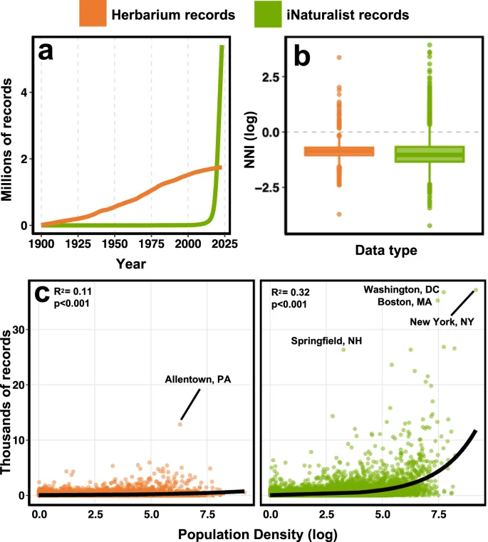
Temporal bias (a) is illustrated as the accumulation of new records over time. Spatial bias (b) is quantified using nearest neighbor index (NNI) which is a measure of spatial autocorrelation. When log transformed, a negative NNI indicates clustering, a positive NNI indicates dispersion, with an NNI of 0 indicating points are randomly distributed in space. NNI was calculated at the species level and only significant (p < 0.05) estimates of NNI were retained for this visualization (n = 2823). Herbarium records exhibited a mean log NNI of −0.88 while the mean for iNaturalist records was significantly (p = 0.006) lower at −0.93 (Table S1). Boxes show the quantiles (Q1-3) with the horizontal line representing the median and the whiskers representing the minima and maxima (calculated as 1.5 times the difference between Q1-3). We also tested for spatial bias (c) by estimating the relationship between density of records and human population density using negative binomial generalized linear models for which we report R2 (Kullback–Leibler) and p values (Tables S2-S3).
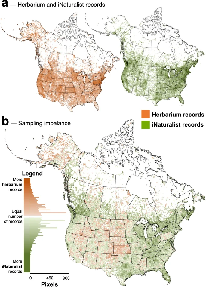
To visualize the spatial distribution, we produced maps of the log density of herbarium and iNaturalist records (a) at 25 km2 resolution for Canadian vascular plants across Canada and the United States. These maps were combined to generate a map of sampling imbalance (b) where orange pixels indicate more herbarium records and green pixels indicate more iNaturalist records. The distribution of sampling imbalance is visualized next to the legend.
When it comes to representing plant diversity, we find that herbarium records are less taxonomically, phylogenetically, and functionally biased. On average, while a single plant species is represented by more iNaturalist observations (µ = 1234) compared to herbarium records (µ = 396), the variance is 4.8 times higher for iNaturalist data (F = 4.776, df = 4391, p < 0.001), which leads to half of all iNaturalist observations (2.7M) representing only 4% (178) of plant species. As a result, 47% of Canadian plants are better represented by herbarium records despite there being considerably fewer compared to iNaturalist observations (Fig. 4a). Pagel’s λ, which measures the strength of signal in the distribution of a trait at the tips of a phylogenetic tree or of a functional dendrogram, is higher for iNaturalist observations compared to herbarium records, indicating stronger phylogenetic and functional bias (Fig. 4b, c).
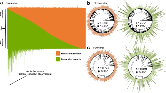
Taxonomic bias (a) is represented as the ratio of herbarium to iNaturalist records for each species of plant, accompanied by bar plots above and below which correspond to the number of herbarium and iNaturalist records for each species respectively. Phylogenetic (b) and functional (c) bias is represented as the number of herbarium and iNaturalist records per plant arranged around the phylogenetic tree or functional dendrogram. To enhance visualization, we took the square root of the number of records. Finally, we tested for bias in the distribution of the number of records per species at the tips of both the phylogenetic tree and functional dendrogram using Pagel’s λ, which varies between 0 and 1 with 0 indicating no bias (number of records per sample randomly distributed across the tree) signal and 1 indicating high bias (number of records per sample are highly correlated with the phylogenetic or functional structures). We assessed significance using likelihood ratio tests and reported p-values.
Taxonomic, phylogenetic, and functional coverage
Despite only having a third as many records in GBIF, herbarium specimens better capture the taxonomic, phylogenetic, and functional diversity of Canadian plants (Fig. 5a–c). Of the 4392 terrestrial vascular plant species in Canada, digitized herbarium specimens represent 3662 (83.4%) compared to the 3504 (79.8%) represented by iNaturalist observations. Species at risk are also better represented, with Herbarium records capturing 93.2% compared to 88.7% for iNaturalist data. Surprisingly, 714 (16.3%) species were unrepresented by either data type. When it comes to phylogenetic and functional coverage, herbarium records capture 3.4% more phylogenetic diversity and 1.8% more functional diversity. Based on the rate at which iNaturalist data accumulate taxonomic, phylogenetic, and functional diversity, we estimate it would take over 4.2M additional iNaturalist observation to capture the diversity currently represented by digitized herbarium specimens.
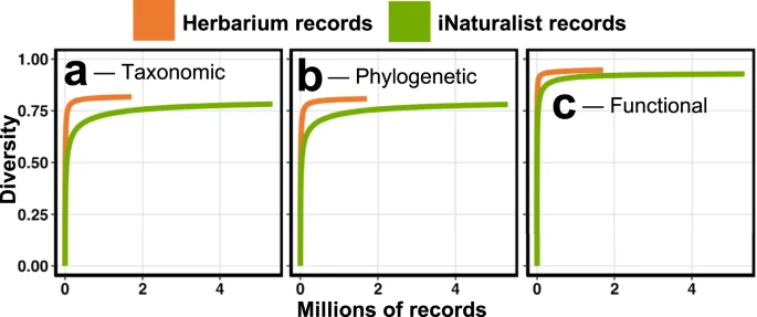
Based on 1000 randomizations, we show that despite only having one-third as many records, herbarium specimens accumulate more taxonomic (a), phylogenetic (b), and functional (c) diversity than iNaturalist observations.
Capturing species’ environmental niches
Using species range maps and current climate normals, we report that the environmental niches of Canadian plants are surprisingly poorly captured by both herbarium and iNaturalist data. Together, both data types capture an average 9.2% of species’ environmental niches. Separately, iNaturalist observations capture an average 5.7% of species environmental niches while herbarium records capture around 5.1%. However, when adjusted for the fact that there are over three times as many iNaturalist records, herbarium records captured an average 1.8 times more environmental niche space per record. This difference is reflected in accumulation curves (Fig. 6a), where herbarium records accumulate environmental niche coverage 9% quicker than iNaturalist data for the average plant species. Interestingly, the proportion of species’ niches captured by both data types was on average very small (1.6%) indicating that the different data types usually capture very different areas within a species’ geographic range.
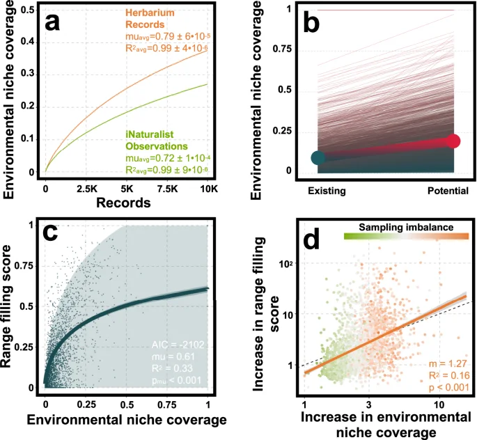
Average niche accumulation curves (a) for herbarium and iNaturalist data show that herbarium records more efficiently capture species’ environmental niches compared to iNaturalist observations. By extrapolating these curves for each species of plant, we estimated the potential niche coverage (b) achievable by digitizing Canada’s remaining 7.3M herbarium records. The large points and thick joining line reflect the existing and potential averages across all species. Using existing niche coverage, we (c) modeled the relationship with our ability to predict species ranges using species distribution models (SDMs), referred to as range filling score (e.g., proportion of species Canadian range predicted by SDMs), using an inflated beta regression (Table S4). Along with the fitted relationship, we also visualized the 95% confidence interval of the curve (darker band) and the prediction interval of the model (lighter band). The fitted curve was used to predict how each species range filling score would increase with the potential increase in niche coverage conferred by digitizing Canada’s remaining herbarium specimens. The potential increase in environmental niche coverage was plotted against the increase in range filling score (d) to illustrate that increasing niche coverage disproportionately increases our ability to model species ranges. To illustrate this further, we fit a simple linear regression (orange line) on the log transformed data (Table S5) to assess whether the slope was significantly greater than 1 (represented by the dashed black line). The shaded area around the line is the 95% confidence interval of the slope based on 2547 degrees of freedom. Points, representing species, are colored based on sampling imbalance between data types.
Benefits of digitizing Canada’s remaining herbarium specimens
An estimated 7.3M specimens remain undigitized in herbaria across Canada19. Assuming that these remaining specimens can be adequately georeferenced and that the taxonomic representation remains like that of digitized specimens, we estimate that the digitization of the remaining records could capture around 156 additional species (3.6%), 5.3% more phylogenetic diversity, and 2.3% more functional diversity. In contrast, it would take an estimated 42M, 41M, and 74M additional iNaturalist records, to capture the same amount of taxonomic, phylogenetic, and functional diversity, respectively.
Based on our analysis of how well herbarium specimens capture species’ environmental niches, we estimate that digitizing Canada’s remaining specimens could almost quadruple existing coverage. While the existing 1.74M herbarium records capture an average 5.1% of species environmental niches, an additional 7.3M records could increase this coverage to 19.8%, which when added to the coverage conferred by existing iNaturalist data, equates to an average niche coverage of around 23.8% across all Canadian vascular plants (Fig. 6b).
Benefits of digitization for modeling the distribution of Canadian flora
The power and usefulness of SDMs to predict species ranges today and into the future under climate change depends on how well the biodiversity observations we use to fit models represent species’ niches. Based on SDMs for Canadian vascular plants, we found a strong positive relationship between niche coverage (the amount of environmental niche space captured in biodiversity data) and our ability to predict the extent of species geographic ranges (range filling score) (Fig. 6c, Table S4). Currently, when using both data types to model Canadian flora, we are only able to predict the occurrence of species across 20.8% of their Canadian range on average, which means we are likely underestimating the true distribution of plant biodiversity across Canada. However, we predict that by digitizing Canada’s remaining herbarium collections, we could increase our ability to model Canadian plant distributions by over 5 times per species on average. Furthermore, our results show that the relationship between increasing the ability of our data to capture species’ niches and the resulting increase in SDM power is likely non-linear, indicating that small improvements in niche coverage translate to disproportionate increases in our ability to model species distributions (Fig. 6d, Table S5).
In contrast, we estimate it would take an additional 27.3M iNaturalist observations to match these benefits of digitization. To put this in perspective, despite the rapid increase in the amount of community science data over the past 5 years, GBIF only contains 78M iNaturalist observations across the entire tree of life (as of January 2024). As such, accumulating this many additional iNaturalist observations for Canadian plants would likely take decades.
Discussion
Our ability to protect biodiversity today and into the future under climate change is underpinned by our ability to predict species distributions, which depends on the availability, amount, and coverage of biodiversity data. Over the past decade, the rise of community science platforms like iNaturalist have changed the way humans interact with nature and provided a windfall of biodiversity observations. But large data gaps persist8, and the extent to which community science has helped overcome the Wallacean shortfall (lack of knowledge of species distributions20) is unclear. Here, we report that iNaturalist observations have significantly increased the diversity and distribution of species captured in online inventories like GBIF. However, in line with past work8, we find that despite having over three times the number of records, iNaturalist data exhibit more bias and capture less taxonomic, phylogenetic, and functional diversity than digitized herbarium specimens. Record-to-record, herbarium specimens also more efficiently describe both plant biodiversity at large as well as the environmental niches of individual species. As such, the digitization of Earth’s remaining natural history collections has the potential to substantially improve both our knowledge of biodiversity as well as our ability to build SDMs that better predict biodiversity today and into the future.
As nations around the world embark on their path to protecting 30% of land by 203012, our ability to integrate climate change planning into the expansion of protected areas may determine the future of Earth’s biodiversity13,14,15. Given the value of already digitized herbarium specimens, our results suggest that the digitization of remaining collections would likely greatly improve our ability to model biodiversity today and into a climatically uncertain future. Moreover, alongside offering valuable (and more scientifically reliable21) species occurrence data, the physical specimen behind the digital record holds a wealth of additional information. In fact, the concept of digitization has recently been extended beyond simple digital images to include layers of additional morphological and genetic data22 that have been used to estimate evolutionary lineages, sample historical genomes, quantify changes in functional traits, uncover new taxa, and re-evaluate what we thought were extinct species23,24,25,26,27,28,29. In the context of global change, herbaria, and their collections are increasingly relied on to understand biodiversity trends in the Anthropocene and provide critical baseline data for future assessments of climate change30,31,32,33,34. This has sparked calls for an open-access global metaherbarium to facilitate the use of herbarium data and realize the immense scientific potential of fully digitized collections25. So why then have only ~21% of Earth’s more than 396M herbarium specimens been digitized10,11?
It is not because herbaria lack the methodological knowledge to do so. Around the world, herbaria are undertaking mass-digitization projects that have resulted in millions of specimens now being digitally available to researchers35,36,37. In Canada, many of the 88 currently active herbaria have digitization experience, and standardized and reproducible digitization workflows are publicly available38,39. Attempts since 2007 to aggregate data under the Canadensys40 network have contributed to the digitization of over 900,000 specimens and have produced a trove of digitization knowledge, resources, and technology. Unfortunately, in Canada and around the world, funding remains a major hurdle to the digitization of remaining specimens10. We estimate that the digitization of Canada’s remaining 7.3M specimens would cost around $22M (~$3 per specimen using traditional workflows35,41,42), which is relatively low when viewed against the biodiversity benefits. For context, in 2023, $22M represented only 0.14% of Canada’s annual spending on science and technology43.
The other major hurdle to mass digitization is the time it takes for specimens to undergo full digitization workflows. While estimates vary greatly, a single herbarium worker can digitize anywhere between 6 and 500 specimens per hour depending on the workflow, complexity of specimen data, level of automation, and capacity of herbarium35,44,45,46,47. Fortunately, the rise of computer vision, artificial intelligence, and high-throughput workflows has the potential to greatly reduce both the cost and time it takes to digitize, while also increasing data standards44,46,48,49,50. For example, the Smithsonian’s US National Herbarium, which houses roughly 3.8M specimens, was recently completely digitized and the use of high-throughput workflows reduced the cost of digitization from $3.32 down to $1.85 per specimen and allowed for the digitization of 3000–4000 specimens daily35. As technologies continue to advance, the digitization of remaining records is not only a potentially effective way to generate valuable biodiversity data but is also increasingly feasible and cost-efficient.
Alongside the digitization of existing records, targeted collection of new herbarium specimens combined with modern geolocating technology, has the potential to rapidly fill gaps in our understanding of biodiversity. For example, targeting species that have been described but are underrepresented in GBIF could help fill Canada’s taxonomic, phylogenetic, and functional data gaps. Likewise, because iNaturalist data poorly capture species niches due to the high spatial bias in sampling location and the taxonomic preference towards common species4,5, targeted collection of rare species in under-sampled regions could rapidly produce disproportionately valuable data for modeling species distributions. One example of such a program is the Canadian Museum of Nature’s Arctic Flora Biodiversity Project51 which aims to increase our knowledge of Arctic plant and lichen biodiversity through systematic collection. The concept of targeted collection can also harness the usefulness of community science platforms52 and initiatives like British Columbia Parks Biodiversity Program53 offer a good example of how informed data collection can leverage public engagement to benefit conservation, research, and biodiversity.
Fundamentally, while we can try to predict the importance of undigitized herbarium collections, we ultimately do not know what hidden value they hold. Until we bring these specimens out of their cabinets and into the digital light, their significance to our understanding of biodiversity will remain unclear30. What is clear is that community science observations are limited in their ability to capture the diversity and distribution of plants and the ongoing rapid accumulation of new observations is unlikely to fill existing data gaps—at least for the next few decades. For this reason, the funding of either large-scale targeted sampling programs or mass digitization initiatives is likely necessary to rapidly improve our understanding of plant biodiversity. And while targeted programs are almost certainly more effective54,55,56, funding Earth’s remaining herbaria offers more than just georeferenced point data. Herbaria operate as critical bridges between the scientific community and the public36,57,58, and represent one of the last refuges for the study of plant taxonomy and systematics25, fields that have been hemorrhaging funding, positions, and representation at universities and even museums worldwide59. As such, empowering our remaining herbaria would not only preserve irreplaceable knowledge, skills, and specimens but might also hold the key to producing the critical biodiversity data we need to predict and protect Earth’s biodiversity now and into the future.
Methods
Ethics and inclusion
The lands that many now call Canada, are the stolen traditional territories of many diverse First Nations, Métis, and Inuit Peoples. We recognize that the 88 remaining herbaria in Canada (and aspects of herbaria globally60) are a product of the colonization and exploitation of land long stewarded by Indigenous Peoples. Many of the specimens housed in herbarium collections were gathered by botanists who used local Indigenous Knowledge often without appropriate recognition. As a result, despite their critical influence, Indigenous voices are largely absent from Canadian herbarium collections. However, some herbaria are taking steps to amplify Indigenous voices, and ongoing initiatives such as Plenty Canada’s Greenbelt Indigenous Botanical Survey61, Canadian Museum of Nature’s Capture the Collections62, and McGill University Herbarium’s Recovering Lost Voices63, demonstrate ways that herbaria can work towards truth and reconciliation in Canada. Moving forward, as herbarium specimens are digitized and made accessible, investigating and communicating the colonial and Indigenous legacies of these collections is critical for both their scientific and societal value.
Species lists and occurrence data
Starting with a full list of Canada’s vascular plants64 we downloaded all the GBIF observations in both Canada and the United States from 1900 to present (January 2024) to enable a contemporary comparison of both iNaturalist and herbarium records65,66. First, GBIF observations with a coordinate uncertainty of over 25 km were removed. Then data were divided into two groups representing iNaturalist records (institution code “iNaturalist”) and herbarium records (basis of record “PRESERVED_SPECIMEN”). This resulted in 5,423,637 research grade iNaturalist observations and 1,742,166 Herbarium records.
Temporal bias
To illustrate temporal bias, we simple plotted the accumulation of herbarium and iNaturalist records annually from 1900 till present (January 2024).
Spatial bias
To test for spatial biases in each data type we used Nearest Neighbor Index (NNI) which is a measure of spatial autocorrelation67. When log transformed, negative NNI indicates that the geographic locations (latitude, longitude) of records are more clustered than expected and positive NNI indicates records are more spread than expected, with an NNI of 0 indicating points are randomly distributed in space. After calculating NNI for each point for each data type, we used a two-sided t-test to test for significant differences between the means. NNI was calculated using the nni() function in the “spatialEco” package for R68. To visualize spatial bias in number of records, we mapped the total number of records per 25 km2 grid cells across Canada and the United States. To visualize the imbalance between herbarium and iNaturalist sampling effort per cell, we mapped the difference between the relative portion of records of each data type. This produced a map that highlights areas of higher iNaturalist observation density compared to herbarium record density and vice versa. Finally, because past work has demonstrated that iNaturalist observations tend to occur in areas of high human population density, we modeled the relationship between number of records and population density across North America for both data types. To do this we used the Gridded Population of the World (v4) raster for the year 202069, downloaded at 2.5 arc-minute resolution (roughly 5 km2). We then resampled this raster to our 25 km2 grid for North America using bilinear resampling in the terra package for R70. Using the rasterized layers of herbarium and iNaturalist record counts, we then assembled a data frame for all cells with at least 1 record of either data type and extracted the corresponding population density value for each cell. Because we are dealing with integer count data, we fit negative-binomial generalized linear models using the MASS package for R71. We log-transformed population density to improve model fit. We report both model parameters, AIC, and pseudo R2 (Kullback–Leibler) calculated with the performance package for R72.
To visualize the spatial distribution of herbarium and iNaturalist records, we rasterized record data at 25 km2 resolution across Canada and the United States. To view the balance between data types across space, we took the difference in number of records per pixel. We overlayed national, provincial, territorial, and state borders73 to aid visualization.
Taxonomic bias
To quantify taxonomic bias, we assessed whether the variance across the number of records per species differed between herbarium and iNaturalist data using an F test. To control for the different number of total records per data type, we used relative number of records to perform the F test.
Phylogenetic and functional bias
To quantify phylogenetic and functional bias we first needed phylogenetic and functional data. We built a phylogenetic tree of Canadian vascular plants using the “rtrees” package for R74. To visualize and assess bias we built a functional dendrogram to match our phylogenetic tree. First, we downloaded the following plant functional traits from the TRY database75: Seed dry mass, Plant height vegetative, Leaf area per leaf dry mass (specific leaf area, SLA or 1/LMA): undefined if petiole is in- or excluded, Plant lifespan (longevity), Plant nitrogen(N) fixation capacity, Plant growth form, Leaf photosynthesis pathway, Dispersal syndrome, Plant reproductive phenology timing, Leaf compoundness, Plant woodiness, Leaf type. These traits were selected based on taxonomic coverage and have been used in the past to capture and represent the functional diversity of Canada’s plants15. Using these traits, we calculated an average trait value for each species of plant and phylogenetically imputed missing values using phylogenetic vector regressions in the “PVR” package for R76 and random forest regression trees in the “missForest” package for R77. Plants with no functional trait data were dropped from the analysis since imputing these species would be solely based on PVR values. This left us with a remaining 4147 (94%) species with complete functional and phylogenetic data. From there, functional traits were used to calculate a Gower’s distance matrix using the “FD” package for R78 which was used to construct a functional dendrogram using UPGMA clustering achieved with the hclust() function in “stats” package included in base R79. Once we had both our phylogenetic tree and functional dendrogram for the remaining 4147 plant species, we used Pagel’s λ which estimates the degree to which shared branch lengths influence the distribution of trait values at the tips of a phylogenetic tree or functional dendrogram80. Values of Pagel’s λ range between zero and one, with zero representing phylogenetic independence and one representing perfect Brownian motion (strong phylogenetic bias). Pagel’s λ has been shown in the past to outperform other estimates of phylogenetic signal81. We chose to use Pagel’s λ to test for both phylogenetic and functional bias to standardize our approach and to allow us to compare the strength in both phylogenetic and functional bias in our data. In our data, bias can be thought of as the evenness of the number of records per species across the phylogenetic tree or functional dendrogram. In this case, a high λ (close to 1) would indicate that the number of records is highly correlated to the phylogenetic or function structure of the tree/dendrogram, meaning that, for example, if one species is represented by a high number of records, more phylogenetically related or functionally similar species are more likely to also be represented by a high number of records compared to a distantly related species. On the other hand, a λ close to 0 would suggest that the number of records is randomly distributed across the phylogenetic tree or functional dendrogram, suggesting that little bias is present in that data type. Pagel’s λ was calculated using the phylosig() function in the “phytools” package for R82 based on the log-transformed (to achieve a normal distribution) number of herbarium and iNaturalist records for each species of plant. Phylogenetic and functional bias were visualized by plotting the square root (instead of log) of these values for each tip in the phylogenetic and functional trees. This was done to enable better visualization of the variation in record number across species.
Taxonomic coverage
Once we had assessed bias, we were interested in quantifying the degree to which herbarium and iNaturalist records captured the full diversity of Canada’s vascular plants. Starting with taxonomic coverage, we first quantified the number and proportion of all Canadian vascular plants represented in each data type. Then, to understand how efficiently each data type captures the taxonomic diversity of Canada’s plants, we built modified species accumulation curves. First, each species in the VASCAN list was assigned a value representing its contribution to the total taxonomic diversity. For taxonomic diversity, this was simply one divided by the number of species. Then, working with iNaturalist and herbarium records separately, we then randomly accumulated records, and for each record added, recorded both the index number (e.g., the 5th record added), the species (e.g., Cypripedium parviflorum), and the proportion of taxonomic diversity represented by that species (e.g., one divided by the total number of species in VASCAN). When the added record (e.g., the 5th randomly selected record) corresponded to a species that was already captured in the accumulation by an earlier record (e.g., the 3rd randomly selected record), the proportion of taxonomic diversity represented by that record was recorded as zero, since that species had already been accounted for. This process was repeated until all records had been added, and the entire process was then repeated 1000 times. From these 1000 runs, we calculated the average proportion of taxonomic diversity captured for each index position for each data type. Using these averages and the corresponding index position, we then fit logarithmic beta regressions83 to these curves to allow us to estimate the increase in niche coverage with the addition of novel records. Traditional species accumulation curves are usually used to quantify sampling completeness or estimate the true number of species in a study region (usually by identifying the asymptote of the accumulation curve). In our case, we know the total number of plant species in Canada (based on the VASCAN list). Because of this, we needed to be able to fit a curve that reflected the fact that eventually, if we accumulate an infinite number of herbarium or iNaturalist records, we should be able to reach (at least asymptotically) the total number of plants in the VASCAN list. Logistic Beta regressions allowed us to do this and by log-transforming the independent variable (number of records) we achieved a logarithmic-shaped curve that reaches an asymptote at 1 as expected under sampling theory. Beta regressions operate with a response variable distributed between 0 and 1 and in this study, we used the proportion of all species as the response instead of the total number of species. The slope of this regression indicates how quickly different datatypes accumulate taxonomic diversity. We fit beta regressions using the “betareg” package for R84.
Phylogenetic coverage
We used phylogenetic coverage to assess how well each data type captures the full phylogeny, representing millions of years of plant evolution in Canada. Using the phylogenetic tree described earlier, we used the evol_distinct() command in the “phyloregion” package for R85 to estimate the relative phylogenetic distinctiveness of each species. Total coverage then, was calculated as the proportion of all phylogenetic distinctiveness captured by each data type. We then built accumulation curves but instead of taxonomic diversity, we accumulated phylogenetic diversity with the addition of new records. To do so we used the same approach as described above and fit the same beta regressions.
Functional coverage
We used functional coverage to assess how well each data type captures Canadian functional diversity, representing the variation in ecological roles played by different species of Canadian plants. Starting with the functional dendrogram described above, we calculated the relative functional distinctiveness of each species again using the evol_distinct() command in the “phyloregion” package for R85. To estimate total coverage, we calculated the proportion of all functional distinctiveness captured by each data type. We then built accumulation curves but instead of accumulating taxonomic diversity, we accumulated functional diversity with the addition of new records. Again, using the same approach and beta regressions as described above.
Niche coverage
To estimate how herbarium and iNaturalist records represent the spatial and environmental niches of plants we first had to calculate the extent of their niche space. To do so we relied on the expertly estimated plant ranges provided as polygons in the BIEN dataset, accessed through the “BIEN” package for R86. Of the 4392 vascular plants in Canada, only 3269 (74%) have estimated range maps, of which only 3174 also had GBIF records. We acknowledge that areas within species range polygons do not always indicate species presence. If analyzed at a fine grain size (e.g., 1 km2), one would expect there to be cells within a species range that are not occupied by that species due to variation in suitable habitat across species ranges. To account for this, we chose a coarse grain size (25 km2) to try and maximize the probability that suitable habitat occurred in each grid cell. Furthermore, the range polygons used in our analysis were not simple convex hulls but contained holes to account for regions within the spatial extent of the range where species are likely not present.
To estimate spatial coverage, we rasterized range maps at the 25 km2 resolution and simply calculated the proportion of raster cells in the species range that had herbarium/iNaturalist records in them. To go from spatial coverage to environmental niche coverage, we needed to estimate the “proportion” of the species environmental niche present in each raster grid cell. Starting with 5 climate normal layers (Mean Annual Precipitation, Precipitation as Snow, Humidity, Degree days above 0°, and Degree days above 18°) downloaded from AdaptWest Project87 spanning the past 30 years, we first aggregated the climate layers up to 25 km2 resolution to match the spatial grid of already rasterized plant ranges. These climate layers were used to match the climate variables used to construct the SDMs used later in the analysis. For each species of plant, we extracted the climate values for all cells within its rasterized range polygon to assemble a cell by climate matrix. To account for differences in measurement scale, we standardized climate variables using decostand() in the “vegan” package for R88. From there we computed a Euclidean distance matrix, which was clustered to form a dendrogram, like our functional dendrogram but clustering cells by climate similarity instead of by species functional traits. Using this climatic dendrogram, we calculated the individual contribution of each cell in said species range to the total climatic niche of that species using the same evol_distinct() command in the “phyloregion” package for R85. Finally, these values, representing the climatic distinctiveness of each 25 km2 cell in a species range were made relative so that the total across all cells in a species ranges summed to 1. This process was repeated for all species, recalculating the climatic distance matrix and climatic dendrogram each time to allow for differences between species based on differences between their realized climatic niches. Another possible approach would have been to decompose our climate variables into 2-dimensional principal component space, to identify geographic areas with similar environmental conditions. However, at coarse grain sizes such as the one we used, we believe it is safe to assume that each geographic pixel represents a unique combination of environmental variables. As such, we chose to instead assign a proportion of environmental niche space to each geographic pixel to give weight to pixels with highly dissimilar combinations of environmental conditions compared to pixels with more similar conditions.
Using these estimates of spatial and environmental coverage per cell, we then built modified accumulation curves to model how rapidly herbarium and iNaturalist records were capturing species niches. First, we removed all herbarium and iNaturalist records found outside of the species rasterized range. Then we assigned each record a cell number corresponding to the 25 km2 grid cell it occurred in. Working with herbarium and iNaturalist records separately, we then randomly accumulated records, and for each record added, recorded both the index number (e.g., the 5th record added), the spatial contribution of that cell (e.g., 1 divided by the number of cells in that species range), and the climatic contribution of that cell (e.g., the relative climatic distinctiveness). When the added record (e.g., the 5th randomly selected record) corresponded to a cell that was already captured in the accumulation by an earlier record (e.g., the 3rd randomly selected record), the spatial and climatic contribution of that record was recorded as zero, since that cell had already been accounted for. This process was repeated until all records had been added, and the entire process was then repeated 1000 times. From these 1000 runs, we calculated the average spatial and environmental contribution of each indexed record for each data type. Using these averages and the corresponding index position, we then fit logarithmic beta regressions to these curves to allow us to estimate the increase in niche coverage with the addition of novel records. While we used both spatial and environmental niches in our analysis, the results were virtually identical, so we chose to report environmental niche results in the main text and figures.
Beta regression fit
For the 3174 plants for which we attempted to fit beta regressions, model fit was very good. Goodness of fit (pseudo-R2) ranged from an average 0.996 (min = 0.898, max = 1) for herbarium regressions to an average 0.991 (min = 0.772, max = 1) for iNaturalist regressions. Because some regressions did not converge and some species were excluded due to too few data points, we chose to report community averages instead of individual species results. Regressions that did not converge were removed from the analysis.
Extrapolating beta regressions
There is an estimated 7.3 million undigitized herbarium specimens housed in active Canadian herbaria19. While the exact number is unknown, this estimate is probably on the lower side, since it only reflects information from herbaria for which metadata are available, including herbarium specimens that have at least been counted and catalogued and does not include the potentially millions of other records that remain hidden away in collections that lack resources to make even their metadata accessible. As such, our use of this number to reflect the potential benefits incurred by the digitization of Canada’s remaining herbarium specimens is likely conservative.
To estimate how the digitization of herbarium records would add taxonomic, phylogenetic, functional, and niche coverage, we used regression coefficients. Then we used curves fit to iNaturalist data to estimate how many additional iNaturalist records would be required to match the added coverage conferred by herbarium digitization. For niche coverage, since there is taxonomic bias in herbarium representation, we first calculated the relative incidence of each species in existing herbarium records on GBIF. This was used to divide the undigitized 7.3M records in Canada into an expected number of undigitized records per species, which was used to estimate the increase in niche coverage using beta regressions. While this approach assumes that no additional species will be present in the undigitized 7.3M records, our other results suggest that an additional 156 species could be found in the undigitized records. However, these species, not represented in already digitized specimens, are likely rare and represented by only a few of the remaining 7.3M undigitized records. One limitation of this approach is that past digitization may have focused on specific clades (e.g., to understand trait variation in a single genus across space or time) and so it is possible that the taxonomic representation in undigitized collections is different than that of digitized specimens. To estimate the number of iNaturalist records required to match potential coverage given digitization, we simply extrapolated the iNaturalist beta regressions.
Translating current and potential niche coverage into benefits for species distribution modelling
We relied on SDMs detailed in Eckert et al. (2023). These models were built using GBIF data downloaded on June 5th, 202189,90 for all Canadian vascular plants. We first thinned observation records down to a single observation per 1 km grid cell in North America. To further clean data points unlikely to represent the native distribution, we removed any points in core urban areas (e.g., areas designated ‘urban or built-up’ in the land-use/land cover data described below), which often included clusters of data points in botanical gardens/zoos/sanctuaries.
We used the following set of climatic variables that were biologically meaningful and had low correlation: mean annual precipitation (mm), chilling degree days (Degree-days below 0 °C), precipitation as snow (mm), Hargreave’s climatic moisture index and warming degree-days above 18 °C. We used current climate models from AdaptWest Project (2021). Current climate data is based on PRISM and WorldClim and spans 1991–2020. We also included topographic wetness index (calculated based on the 1-km) digital elevation model using package “dynatopmodel” in R91, topographic ruggedness index (from AdaptWest), and an aggregated land cover layer based on MODIS land cover data and reprojected to our grid and reclassified to: unvegetated, hardwood forests, evergreen forest, mixed forests, shrubs, and grasslands92. Finally, we used three variables to represent soil properties (topsoil silt fraction, subsoil pH, and topsoil organic C content) from the Unified North American Soil Map93 (0.25 degree resolution) that were projected to match the 1-km2 climate raster.
We fit Boosted Regression Trees (BRTs)94,95,96 with all environmental, topographic, and soil predictors in the “dismo” package for R97. All presences were used in the models unless they exceeded 5000, in which case 5000 presences were randomly drawn along with 10,000 absences. BRTs were projected across all North America, although only the Canadian ranges were used in subsequent analyses. Model outputs were used to estimate the degree to which our SDMs can “fill” expertly estimated species range maps from the BIEN package86. To do so, we first aggregated projections (keeping the maximum value) to 25 km and thresholded at 0.5 to identify areas where presence is highly likely. While it is unrealistic to expect any single species to occupy the entire extent of its spatial range, once aggregated to a coarse 25 km2 resolution, we operated under the assumption that within a species range boundary, there is likely suitable habitat in each 25 km2 subdivision, which we accounted for by retaining the maximum predicted probability of occurrence during aggregation. We then calculated the number of grid cells in the BIEN range that predicted a presence versus the number of grid cells in the entire range to estimate range filling. For example, if a species was predicted to be present in 10 grid cells in its BIEN range of 100 grid cells, then its range-filling score is 0.1.
To estimate how increased niche coverage might impact the ability of our SDMs to fill species ranges, we needed to model the relationship between current niche coverage and range filling. Since range-filling scores were distributed between 0 and 1 (representing the proportion of the species range filled by our SDMs) we again used a beta regression. Because some species had either none or all of their range filled by our models, and traditional beta distributions do not handle 0 s and 1 s, we used an inflated beta distribution (family=BEINF) and logit link functions to fit a Generalized Additive Model for Location Scale and Shape (GAMLSS) in the “gamlss” package for R98 (Table S4). To improve model fit we used the square root of niche coverage as our predictor variable. Model estimates are provided in Table S1. Instead of using the fitted µ curve to generate a single mean estimate of potential gain in predictive power, we used the curve to estimate potential gain for each species of plant, predicting values using potential niche coverage. The average across all plants (including species represented by 0 or 1) is reported in the main text and visualized in Fig. 6b. Finally, to understand how increasing the niche coverage translates to increases in range-filling scores we fit a simple linear regression on log-transformed data (Table S5).
Estimating the cost of digitization
To estimate how much it costs herbaria to digitize a single specimen, we consulted the curators of major herbaria in Canada along with past work and reports from other herbaria around the world. This estimate of $3 per specimen represents the use of traditional workflows involving cameras and humans and does not account for new high-throughput workflows that are largely automated but initially costly to install.
Reporting summary
Further information on research design is available in the Nature Portfolio Reporting Summary linked to this article.
Data availability
All publicly accessible data is cited and can be downloaded from their respective repositories. The data used and generated in this study have been deposited in Figshare under accession code https://doi.org/10.6084/m9.figshare.25180595.v2. This includes all data needed to reproduce the analysis and figures. Sources of raw data used in this study are available in Table S6 in the Supplementary Information. Source data are provided with this paper.
Code availability
Annotated code to reproduce the analyses and figures is available in the same Figshare repository (https://doi.org/10.6084/m9.figshare.25180595.v2).
References
-
Waller, J. Will citizen science take over? data blog. https://data-blog.gbif.org/post/gbif-citizen-science-data/ (2019).
-
García-Roselló, E., González-Dacosta, J. & Lobo, J. M. The biased distribution of existing information on biodiversity hinders its use in conservation, and we need an integrative approach to act urgently. Biol. Conserv. 283, 110118 (2023).
Google Scholar
-
Grand, J., Cummings, M. P., Rebelo, T. G., Ricketts, T. H. & Neel, M. C. Biased data reduce efficiency and effectiveness of conservation reserve networks. Ecol. Lett. 10, 364–374 (2007).
Google Scholar
-
Callaghan, C. T., Poore, A. G. B., Hofmann, M., Roberts, C. J. & Pereira, H. M. Large-bodied birds are over-represented in unstructured citizen science data. Sci. Rep. 11, 19073 (2021).
Google Scholar
-
Geurts, E. M., Reynolds, J. D. & Starzomski, B. M. Turning observations into biodiversity data: broadscale spatial biases in community science. Ecosphere 14, e4582 (2023).
Google Scholar
-
James, S. A. et al. Herbarium data: global biodiversity and societal botanical needs for novel research. Appl. Plant Sci. 6, e1024 (2018).
Google Scholar
-
Panchen, Z. A., Doubt, J., Kharouba, H. M. & Johnston, M. O. Patterns and biases in an Arctic herbarium specimen collection: Implications for phenological research. Appl. Plant Sci. 7, e01229 (2019).
Google Scholar
-
Daru, B. H. & Rodriguez, J. Mass production of unvouchered records fails to represent global biodiversity patterns. Nat. Ecol. Evol. 7, 816–831 (2023).
Google Scholar
-
Greve, M. et al. Realising the potential of herbarium records for conservation biology. S. Afr. J. Bot. 105, 317–323 (2016).
Google Scholar
-
Paton, A. et al. Plant and fungal collections: current status, future perspectives. Plants People Planet 2, 499–514 (2020).
Google Scholar
-
Thiers, B. Index herbariorum (The New York Botanical Garden, 2020).
-
United Nations Convention on Biological Diversity, Kunming-Montreal Global Biodiversity Framework (CBD/COP/15/L.25) (Convention on Biological Diversity, 2022).
-
Dobrowski, S. Z. et al. Protected-area targets could be undermined by climate change-driven shifts in ecoregions and biomes. Commun. Earth Environ. 2, 198 (2021).
Google Scholar
-
Schuster, R. et al. Protected area planning to conserve biodiversity in an uncertain future. Conserv. Biol. https://doi.org/10.1101/2022.11.18.517054 (2022).
-
Eckert, I., Brown, A., Caron, D., Riva, F. & Pollock, L. J. 30×30 biodiversity gains rely on national coordination. Nat. Commun. 14, 7113 (2023).
Google Scholar
-
Araújo, M. B. & Guisan, A. Five (or so) challenges for species distribution modelling. J. Biogeogr. 33, 1677–1688 (2006).
Google Scholar
-
Kramer‐Schadt, S. et al. The importance of correcting for sampling bias in MaxEnt species distribution models. Divers. Distrib. 19, 1366–1379 (2013).
Google Scholar
-
Meynard, C. N., Leroy, B. & Kaplan, D. M. Testing methods in species distribution modelling using virtual species: what have we learnt and what are we missing? Ecography 42, 2021–2036 (2019).
Google Scholar
-
Bruneau, A., Sinou, S. & Tudor, S. Herbarium digitisation in Canada. Can. Bot. Assoc. Bull. 35, 37 (2020).
-
Lomolino, M. V. Conservation biogeography. in Frontiers of Biogeography: New Directions in the Geography of Nature, vol. 293 (Sinauer Associates, 2004).
-
Aceves‐Bueno, E. et al. The accuracy of citizen science data: a quantitative review. Bull. Ecol. Soc. Am. 98, 278–290 (2017).
Google Scholar
-
Hedrick, B. P. et al. Digitization and the future of natural history collections. BioScience 70, 243–251 (2020).
Google Scholar
-
Albani Rocchetti, G. et al. Reversing extinction trends: new uses of (old) herbarium specimens to accelerate conservation action on threatened species. N. Phytologist 230, 433–450 (2021).
Google Scholar
-
Bebber, D. P. et al. Herbaria are a major frontier for species discovery. Proc. Natl Acad. Sci. US. 107, 22169–22171 (2010).
Google Scholar
-
Davis, C. C. The herbarium of the future. Trends Ecol. Evol. 38, 412–423 (2023).
Google Scholar
-
Folk, R. A. et al. High‐throughput methods for efficiently building massive phylogenies from natural history collections. Appl. Plant Sci. 9, e11410 (2021).
-
Kothari, S., Beauchamp‐Rioux, R., Laliberté, E. & Cavender‐Bares, J. Reflectance spectroscopy allows rapid, accurate and non‐destructive estimates of functional traits from pressed leaves. Methods Ecol. Evol. 14, 385–401 (2023).
Google Scholar
-
Nic Lughadha, E. et al. The use and misuse of herbarium specimens in evaluating plant extinction risks. Philos. Trans. R. Soc. B 374, 20170402 (2019).
Google Scholar
-
Ramirez‐Parada, T. H., Park, I. W. & Mazer, S. J. Herbarium specimens provide reliable estimates of phenological responses to climate at unparalleled taxonomic and spatiotemporal scales. Ecography 2022, e06173 (2022).
Google Scholar
-
Johnson, K. G. et al. Climate change and biosphere response: unlocking the collections vault. BioScience 61, 147–153 (2011).
Google Scholar
-
Lang, P. L. M., Willems, F. M., Scheepens, J. F., Burbano, H. A. & Bossdorf, O. Using herbaria to study global environmental change. N. Phytologist 221, 110–122 (2019).
Google Scholar
-
Lister, A. M. Natural history collections as sources of long-term datasets. Trends Ecol. Evol. 26, 153–154 (2011).
Google Scholar
-
Meineke, E. K., Davis, C. C. & Davies, T. J. The unrealized potential of herbaria for global change biology. Ecol. Monogr. 88, 505–525 (2018).
Google Scholar
-
Meineke, E. K., Davies, T. J., Daru, B. H. & Davis, C. C. Biological collections for understanding biodiversity in the Anthropocene. Philos. Trans. R. Soc. B 374, 20170386 (2019).
Google Scholar
-
Zorich, D. The Digitization of the US National Herbarium – Done! | Digitization Program Office. SI Digi Blog https://dpo.si.edu/blog/digitization-us-national-herbarium-done (2022).
-
Borsch, T. et al. A complete digitization of German herbaria is possible, sensible and should be started now. RIO 6, e50675 (2020).
Google Scholar
-
Mandrioli, M. From dormant collections to repositories for the study of habitat changes: the importance of herbaria in modern life sciences. Life 13, 2310 (2023).
Google Scholar
-
Canadensys. Digitization and imaging https://www.canadensys.net/resources/documents/#digitization-and-imaging (2024).
-
iDigBio. Digitization resources https://www.idigbio.org/wiki/index.php/Digitization_Resources (2021).
-
Canadensys. https://www.canadensys.net/.
-
FLAS. Estimated cost of flas services and supplies. University of Florida – Florida Museum https://web.archive.org/web/20240403174322/https://www.floridamuseum.ufl.edu/herbarium/policies/cost-of-services/ (2022).
-
Granzow-de La Cerda, Í. & Beach, J. H. Semi‐automated workflows for acquiring specimen data from label images in herbarium collections. TAXON 59, 1830–1842 (2010).
Google Scholar
-
Statistics Canada. Federal Science Expenditures and Personnel, Activities in the Social Sciences and Natural Sciences (2023).
-
Harris, K. M. & Marsico, T. D. Digitizing specimens in a small herbarium: a viable workflow for collections working with limited resources. Appl. Plant Sci. 5, 1600125 (2017).
Google Scholar
-
Tulig, M., Tarnowsky, N., Bevans, M., Kirchgessner, A. & Thiers, B. Increasing the efficiency of digitization workflows for herbarium specimens. Zookeys 209, 103–113 (2012).
Google Scholar
-
Sweeney, P. W. et al. Large–scale digitization of herbarium specimens: development and usage of an automated, high–throughput conveyor system. TAXON 67, 165–178 (2018).
Google Scholar
-
Lohonya, K., Livermore, L. & Penn, M. Georeferencing the Natural History Museum’s Chinese type collection: of plateaus, pagodas and plants. BDJ 8, e50503 (2020).
Google Scholar
-
Hussein, B. R., Malik, O. A., Ong, W.-H. & Slik, J. W. F. Applications of computer vision and machine learning techniques for digitized herbarium specimens: a systematic literature review. Ecol. Inform. 69, 101641 (2022).
Google Scholar
-
Guralnick, R. et al. Humans in the loop: community science and machine learning synergies for overcoming herbarium digitization bottlenecks. Appl. Plant Sci. 12, e11560 (2024).
Google Scholar
-
Thompson, K. M., Turnbull, R., Fitzgerald, E. & Birch, J. L. Identification of herbarium specimen sheet components from high‐resolution images using deep learning. Ecol. Evol. 13, e10395 (2023).
Google Scholar
-
Arctic Flora Biodiversity – Canadian Museum of Nature. Canadian Museum of Nature https://nature.ca/en/our-science/research-projects/arctic-flora-biodiversity/ (2024).
-
Tulloch, A. I. T., Possingham, H. P., Joseph, L. N., Szabo, J. & Martin, T. G. Realising the full potential of citizen science monitoring programs. Biol. Conserv. 165, 128–138 (2013).
Google Scholar
-
BC Parks Biodiversity Program. BC Parks Biodiversity Program https://www.bcinat.com/ (2021).
-
Navarro, L., Fernández, N. & Pereira, H. The GEO BON approach to globally coordinated biodiversity monitoring. in Proc. 5th European Congress of Conservation Biology (Jyvaskyla University Open Science Centre, Jyväskylä, Finland, 2018). https://doi.org/10.17011/conference/eccb2018/108135.
-
Nuñez‐Penichet, C. et al. Selection of sampling sites for biodiversity inventory: Effects of environmental and geographical considerations. Methods Ecol. Evol. 13, 1595–1607 (2022).
Google Scholar
-
Valdez, J. W. et al. The undetectability of global biodiversity trends using local species richness. Ecography https://doi.org/10.1111/ecog.06604 (2023).
Google Scholar
-
Soteropoulos, D. L. & Marsico, T. D. Community science success for herbarium transcription in Arkansas: building a network of students and volunteers for notes from nature. Castanea 87, 54–74 (2022).
-
Wen, J., Ickert‐Bond, S. M., Appelhans, M. S., Dorr, L. J. & Funk, V. A. Collections‐based systematics: Opportunities and outlook for 2050. J. Syts. Evol. 53, 477–488 (2015).
Google Scholar
-
Wheeler, Q. Are reports of the death of taxonomy an exaggeration? N. Phytologist 201, 370–371 (2014).
Google Scholar
-
Park, D. S. et al. The colonial legacy of herbaria. Nat. Hum. Behav. 7, 1059–1068 (2023).
Google Scholar
-
Greenbelt Indigenous Botanical Survey Launches! Plenty Canada http://www.plentycanada.com/1/post/2023/12/greenbelt-indigenous-botanical-survey-launches.html
-
Capture the Collections. Canadian Museum of Nature https://nature.ca/en/learn-explore/activities/capture-collections/.
-
Recovering Lost Voices. Hidden Hands in Colonial Natural Histories https://hiddenhands.ca/canada/ (2022).
-
Brouillet, L. et al. Database of vascular plants of Canada (VASCAN). Online. (2010).
-
GBIF. Occurrence Download. 1380345621 The Global Biodiversity Information Facility https://doi.org/10.15468/DL.6FJT8Y (2024).
-
GBIF. Occurrence Download. 396343141 The Global Biodiversity Information Facility https://doi.org/10.15468/DL.TAKS2V (2024).
-
Clark, P. J. & Evans, F. C. Distance to nearest neighbor as a measure of spatial relationships in populations. Ecology 35, 445–453 (1954).
Google Scholar
-
Evans, J. & Murphy, M. spatialEco. (2023).
-
Center For International Earth Science Information Network-CIESIN-Columbia University. Gridded Population of the World, Version 4 (GPWv4): Population Density, Revision 11. Palisades, NY: Socioeconomic Data and Applications Center (SEDAC) https://doi.org/10.7927/H49C6VHW (2017).
-
Hijmans, R. J. et al. Package ‘terra’ (Maintainer: Vienna, Austria, 2022).
-
Venables, W. N. & Ripley, B. D. Modern Applied Statistics with S. (Springer, New York, NY, 2002). https://doi.org/10.1007/978-0-387-21706-2.
-
Lüdecke, D., Ben-Shachar, M., Patil, I., Waggoner, P. & Makowski, D. performance: an R package for assessment, comparison and testing of statistical models. JOSS 6, 3139 (2021).
Google Scholar
-
Commission for Environmental Cooperation. Political boundaries (2021).
-
Li, D. rtrees: an R package to assemble phylogenetic trees from megatrees. Ecography 2023, e06643 (2023).
Google Scholar
-
Fraser, L. H. TRY—A plant trait database of databases. Glob. Change Biol. 26, 189–190 (2020).
Google Scholar
-
Santos, T. PVR: Phylogenetic eigenvectors regression and phylogentic signal-representation curve (2018).
-
Stekhoven, D. J. & Buhlmann, P. MissForest-non-parametric missing value imputation for mixed-type data. Bioinformatics 28, 112–118 (2012).
Google Scholar
-
Laliberté, E., Legendre, P. & Shipley, B. Package ‘FD’ for R. (2014).
-
R Core Team. R: A Language and Environment for Statistical Computing (R Foundation for Statistical Computing, 2023).
-
Pagel, M. Inferring the historical patterns of biological evolution. Nature 401, 877–884 (1999).
Google Scholar
-
Münkemüller, T. et al. How to measure and test phylogenetic signal. Methods Ecol. Evol. 3, 743–756 (2012).
Google Scholar
-
Revell, L. J. phytools: an R package for phylogenetic comparative biology (and other things). Methods Ecol. Evol. 3, 217–223 (2012).
Google Scholar
-
Geissinger, E. A., Khoo, C. L. L., Richmond, I. C., Faulkner, S. J. M. & Schneider, D. C. A case for beta regression in the natural sciences. Ecosphere 13, e3940 (2022).
Google Scholar
-
Cribari-Neto, F. & Zeileis, A. Beta Rregression in R. J. Stat. Soft. 34, 1–24 (2010).
-
Daru, B. H., Karunarathne, P. & Schliep, K. phyloregion: R package for biogeographical regionalization and macroecology. Methods Ecol. Evol. 11, 1483–1491 (2020).
Google Scholar
-
Maitner, B. S. et al. The BIEN R package: a tool to access the Botanical Information and Ecology Network (BIEN) database. Methods Ecol. Evol. 9, 373–379 (2018).
Google Scholar
-
AdaptWest Project. Gridded Current and Projected Climate Data for North America at 1km Resolution, Generated Using the ClimateNA v7.01 Software (T. Wang et al., 2021). adaptwest.databasin.org (2021).
-
Oksanen, A. J. et al. Package ‘ vegan’. CRAN Repository 0–291 (2013).
-
GBIF.org. Occurrence Download. 525916669 The Global Biodiversity Information Facility https://doi.org/10.15468/DL.897YAH (2021).
-
GBIF.org. Occurrence Download. 165004383 The Global Biodiversity Information Facility https://doi.org/10.15468/DL.G424JV (2021).
-
Metcalfe, P., Beven, K. & Freer, J. Dynamic TOPMODEL: a new implementation in R and its sensitivity to time and space steps. Environ. Model. Softw. 72, 155–172 (2015).
Google Scholar
-
Friedl, M. A. et al. MODIS Collection 5 global land cover: Algorithm refinements and characterization of new datasets. Remote Sens. Environ. 114, 168–182 (2010).
Google Scholar
-
Liu, S. et al. The Unified North American Soil Map and its implication on the soil organic carbon stock in North America. Biogeosciences 10, 2915–2930 (2013).
Google Scholar
-
Elith, J., Leathwick, J. R. & Hastie, T. A working guide to boosted regression trees. J. Anim. Ecol. 77, 802–813 (2008).
Google Scholar
-
Hijmans, R. J. & Elith, J. Species Distribution Modeling with R (R Cran Project, 2013).
-
Valavi, R., Elith, J., Lahoz‐Monfort, J. J. & Guillera‐Arroita, G. Modelling species presence‐only data with random forests. Ecography 44, 1731–1742 (2021).
Google Scholar
-
Hijmans, R. J., Phillips, S., Leathwick, J., Elith, J. & Hijmans, M. R. J. Package ‘dismo’. Circles 9, 1–68 (2017).
-
Rigby, R. A. & Stasinopoulos, D. M. Generalized additive models for location, scale and shape. J. R. Stat. Soc. Ser. C Appl. Stat. 54, 507–554 (2005).
Google Scholar
Acknowledgements
The authors would like to thank the Canadian Society for Ecology and Evolution and the Canadian Botanical Association for hosting a symposium on the future of herbarium collections from which this work was inspired. The authors would also like to acknowledge members of the Canadensys network for their tireless efforts coordinating the digitization of Canadian herbarium collections. This work was supported by NSERC Discovery Grant RGPIN-2019-05771 (L.J.P.) and by a NSERC CGS-D award (I.E.).
Author information
Authors and Affiliations
Contributions
All authors conceived the idea for the manuscript and helped developed the methodology which was executed by I.E. Results were generated, interpreted with the help of S.J., and visualized by I.E. I.E. wrote the first draft of the manuscript and all authors provided critical feedback. L.J.P. supervised the project and acquired the funding. A.B., D.A.M., and T.A.D. provided expertise and resources relating to the extent of Canada’s undigitized collections as well as the cost of digitization.
Corresponding author
Ethics declarations
Competing interests
The authors declare no competing interests.
Peer review
Peer review information
Nature Communications thanks Lorenzo Peruzzi and the other, anonymous, reviewer(s) for their contribution to the peer review of this work. A peer review file is available.
Additional information
Publisher’s note Springer Nature remains neutral with regard to jurisdictional claims in published maps and institutional affiliations.
Supplementary information
Supplementary Information
Peer Review File
Reporting Summary
Source data
Source data
Rights and permissions
Open Access This article is licensed under a Creative Commons Attribution-NonCommercial-NoDerivatives 4.0 International License, which permits any non-commercial use, sharing, distribution and reproduction in any medium or format, as long as you give appropriate credit to the original author(s) and the source, provide a link to the Creative Commons licence, and indicate if you modified the licensed material. You do not have permission under this licence to share adapted material derived from this article or parts of it. The images or other third party material in this article are included in the article’s Creative Commons licence, unless indicated otherwise in a credit line to the material. If material is not included in the article’s Creative Commons licence and your intended use is not permitted by statutory regulation or exceeds the permitted use, you will need to obtain permission directly from the copyright holder. To view a copy of this licence, visit http://creativecommons.org/licenses/by-nc-nd/4.0/.
Reprints and permissions
About this article
Cite this article
Eckert, I., Bruneau, A., Metsger, D.A. et al. Herbarium collections remain essential in the age of community science.
Nat Commun 15, 7586 (2024). https://doi.org/10.1038/s41467-024-51899-1
-
Received: 13 February 2024
-
Accepted: 08 August 2024
-
Published: 31 August 2024
-
DOI: https://doi.org/10.1038/s41467-024-51899-1
Comments
By submitting a comment you agree to abide by our Terms and Community Guidelines. If you find something abusive or that does not comply with our terms or guidelines please flag it as inappropriate.