Abstract
The efficiency of nanoscale nonlinear elements in photonic integrated circuits is hindered by the physical limits to the nonlinear optical response of dielectrics, which cannot be engineered as it is a fundamental material property. Here, we experimentally demonstrate that ultrafast optical nonlinearities in doped semiconductors can be engineered and can easily exceed those of conventional undoped dielectrics. The electron response of heavily doped semiconductors acquires in fact a hydrodynamic character that introduces nonlocal effects as well as additional nonlinear sources. Our experimental findings are supported by a comprehensive computational analysis based on the hydrodynamic model. In particular, by studying third-harmonic generation from plasmonic nanoantenna arrays made out of heavily n-doped InGaAs with increasing levels of free-carrier density, we discriminate between hydrodynamic and dielectric nonlinearities. Most importantly, we demonstrate that the maximum nonlinear efficiency as well as its spectral location can be engineered by tuning the doping level. Crucially, the maximum efficiency can be increased by almost two orders of magnitude with respect to the classical dielectric nonlinearity. Having employed the common material platform InGaAs/InP that supports integrated waveguides, our findings pave the way for future exploitation of plasmonic nonlinearities in all-semiconductor photonic integrated circuits.
Near-field enhancement of optical second harmonic generation in hybrid gold–lithium niobate nanostructures
Nonlinear and quantum photonics using integrated optical materials
Light-induced symmetry breaking for enhancing second-harmonic generation from an ultrathin plasmonic nanocavity
Introduction
Nonlinear optics has been historically dominated by experimental configurations where interacting optical beams propagate for distances much longer than the involved wavelengths in bulk nonlinear optical crystals1, in optical fibers2, or in integrated photonic waveguides3. More recently, nonlinear metasurfaces, or nanoantenna arrays of subwavelength thickness4 have been introduced to eliminate phase-matching constraints5, leading in the latter case to the emergence of nonlinear plasmonics6,7,8. Plasmonic nanoantennas are often used as a sub-wavelength field concentrator to enhance the interaction between light and nonlinear dielectric systems and molecules9,10,11. Remarkably, it has been shown that the plasmonic nanostructure itself can also provide a sub-diffraction limit source of optical nonlinearity6. However, the mechanism at the origin for this phenomenon is still not fully understood and remains unexploited.
One can identify at least two fundamental mechanisms for instantaneous (i.e. faster than an optical cycle) nonlinear optical response of a plasmonic structure. The first is the dielectric nonlinearity of the bulk material which can be enhanced by the local plasmonic field enhancement (nonlinear dielectric susceptibilities χ(2), χ(3), etc.). The second mechanism is due to the collective motion of free electrons under an external radiation field. Such nonlocal oscillation is ultimately related to the kinetic energy of the free-electron gas and can be modeled by a set of hydrodynamic equations of motion in analogy with a classical fluid. The distinction between these two mechanisms is crucial since there is a physical limit to the maximum dielectric nonlinearity, related to the form of anharmonic potentials12 that sets upper bounds for χ(2) and χ(3). Such limitation however does not apply to free-electron nonlinearities1. Therefore, one may ask whether the free-electron nonlinearity is the dominant effect, and if so, whether it can be harnessed to exceed the limited efficiency of conventional dielectric nonlinearity. Even though the response of a perfectly homogeneous electron gas is intrinsically nonlinear, extracting (i.e. coupling to the far-field) and enhancing nonlinear effects requires nanostructuring the free-electron host medium. In principle, the mere existence of a sharp interface between the host medium and a vacuum could suffice13, but in practice much stronger electron density gradients are obtained in nanoantennas under electromagnetic excitation.
In noble metals, and especially in nanoantenna systems, it is extremely difficult to separately investigate the dielectric and free-electron contributions to nonlinearity, as they coexist everywhere in the solid. Doped semiconductors, on the other hand, offer the possibility of controlling the carrier density via external doping, or via a field-effect gate14,15,16, thus allowing to tune the free-electron response while keeping the dielectric nonlinearity constant.
In this work, we combine experiments and theoretical modeling to demonstrate that free electron contributions can dramatically enhance the nonlinear optical response of heavily doped semiconductor nanoantennas. By measuring third harmonic generation (THG) from nanoantennas with different free-electron density and comparing the obtained efficiency to hydrodynamic model calculations, we unveil that the nonlocal free-electron interaction is the fundamental mechanism of nonlinear plasmonics in doped semiconductors. The material platform employed for the experiment is InGaAs/InP because of its broad appeal for the future exploitation of plasmonic nonlinearities in all-semiconductor photonic integrated circuits (PICs)17,18,19.
Results
The fermionic nature of electron–electron interactions manifests itself as an internal pressure in the electron gas that resists the compression induced by an external electromagnetic field. The effects of such pressure are most apparent near the interfaces between the host material and vacuum or other materials, where strong gradients of the carrier concentration and of the electric field occur. Free-electron nonlinearities8 are therefore intrinsically nonlocal, in the sense that the induced currents depend not only on the value of the electric field at a given point but also, through their spatial derivatives, on the value of the fields in the surrounding area20,21,22. The many-body nonlinear and nonlocal dynamics of a free-electron fluid under external electric and magnetic fields, E(r, t) and H(r, t), is described by the following equation for the electron n(r, t) and current J(r, t) densities23,24,25,26:
where μ0 is the magnetic permeability of vacuum, e is the electron charge, γ is the damping rate of free carrier motion and m* is the electron effective mass that accounts for the band structure in a real solid. The last term on the right-hand side contains the gradient of the functional derivative of the free-energy functional G[n], i.e., the quantum pressure in the electron fluid13,27, which can also be obtained from the Thomas–Fermi screening14. Here we are neglecting the spatial dependence of n at the interface with vacuum(spill-out effect), since the structures we will investigate are relatively large (~1 μm). Following a perturbation approach, it is possible to derive all nonlinear source terms, see details in Supplementary Information (SI)13,14,27,28. Here, we report the two THG source terms that appear in the propagating-wave solution of Maxwell’s equations and Eq. (1): the third-order dielectric polarization ({{bf{P}}}_{{rm{d}}}^{(3)}), and the hydrodynamic contribution S(3) given by the sum of convective and quantum pressure terms:
where Eω and Pω = − Jω/iω are the field and total polarization vectors at the fundamental frequency ω and (beta =sqrt{frac{3}{5}}{v}_{{rm{F}}}), where vF is the Fermi velocity. One immediately sees that an effective hydrodynamic susceptibility cannot be rigorously defined: the additional source ({{bf{S}}}_{3omega }^{(3)}) contains the gradient and the divergence of Pω and therefore it is strictly nonlocal and proportional to (1/{{n}_{0}}^{2}). Paradoxically, in noble metals, the high concentration of free-carrier leads to weaker nonlinear contributions. One can understand this behavior considering the material volume that contributes to the nonlinearity: in metals, the polarization gradients are sharp and non-vanishing only at the metal/vacuum interface, resulting in small active nonlinear volumes; in doped semiconductors, the polarization inhomogeneities extend significantly towards the bulk of the material, leading to a much larger active nonlinear volume (V={l}^{3} sim {({v}_{{rm{F}}}/{omega }_{{rm{p}}})}^{3}propto 1/({n}_{0}^{1/2}{m}^{* 3/2})), where ωp is the plasma frequency21,29. Therefore, the small effective masses m* ~ 0.1me of electrons in semiconductors and their comparatively low carrier density lead to an increased active volume, and eventually to a higher global efficiency, of nonlinearity if compared to noble metals. In the absence of spatial variations of Pω, the nonlinear source term of Eq. (2) vanishes and the hydrodynamic model reduces to the Drude model with the permittivity ({varepsilon }_{{rm{r}}}={varepsilon }_{infty }left(1-frac{{omega }_{{rm{p}}}^{2}}{{omega }^{2}+igamma omega }right)), with the plasma frequency ({omega }_{{rm{p}}}=sqrt{{n}_{0}{e}^{2}/{varepsilon }_{0}{varepsilon }_{infty }{m}^{* }}), where ε∞ is the infinity dielectric constant of the semiconductor (see SI). The plasma wavelength ({lambda }_{{rm{p}}}=frac{2pi c}{{omega }_{{rm{p}}}}) will be used throughout this article, with c being the speed of light in vacuum.
Heavily doped semiconductors display a broad range of λp values in the infrared (IR) spectrum depending on ε∞, m* and n0. In practice, if one restricts to small m* materials compatible with modern PIC nanofabrication processes, the choice reduces to Ge or SiGe grown on Si (group-IV)30, In0.53Ga0.47As grown on InP (InGaAs/InP), and InAs0.9Sb0.1 grown on GaSb (III-V)31. All these material systems allow for a limited dopant incorporation which in practice bounds λp > 5 μm, i.e., to the mid-IR. In this work, we have used electron-doped InGaAs/InP with various dopant densities (m* = 0.041me, ε∞ = 12, n0 ≤ 1 × 1019 cm−3), and utilized fundamental fields (FF) with center wavelength λFF ranging from 12 to 6 μm to drive the nonlinearity. InP has a bandgap energy around 1.35 eV, i.e. absorption edge around 950 nm, which makes it perfectly suitable for infrared applications including supporting PICs (index of refraction 3.1 in the mid-IR).
Three InGaAs films with different doping levels were grown on undoped InP substrates (see Methods). The InGaAs permittivity εr(ω) = ε1 + iε2 was retrieved from the absolute thick-film (~3 μm) reflectivity measured by Fourier-transform infrared spectroscopy (FTIR) using the Kramers-Kroenig relations (Fig. 1c). A Drude fit to εr(ω) provides n0 = 1.02 × 10¹⁹, 8.6 × 10¹⁸ and 5.9 × 1018 cm−3, for samples 1, 2, and 3 respectively, and a doping-independent scattering rate γ0 = 8.9 THz. λp = 7.33, 7.97, and 9.62 μm were directly obtained as the zero-crossing point of ε1 in Fig. 1c32. Photo-excitation of electron–hole plasmas in undoped semiconductors is an alternative method to study even higher free-electron density plasmas, but the temporal33 and spatial34 dynamics are more complex and may obscure the hydrodynamic behavior of free electrons. The InGaAs nanoantennas, consisting of periodically arranged rectangular rods with slightly trapezoidal cross-sections, have been fabricated by etching the excess InGaAs down to the InP substrate by deep reactive ion etching (RIE) through a mask produced by electron-beam lithography, as shown in Fig. 1b. As anticipated in the introduction, the choice to conduct the experiment using rectangular antennas instead of a thin film, which is also feasible (see SI), was made to enhance the differences between dielectric nonlinear susceptibility χ(3) and the hydrodynamic nonlinearity due to the much larger volume with significant polarization gradients.
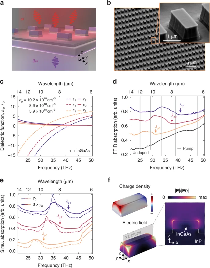
a Schematic illustration of the InGaAs plasmonic antenna on dielectric InP, and the nonlinear experiment producing third harmonic radiations. b Scanning electron microscope image of the antennas, featuring length, width and thickness approximately equal to 2.2 μm, 0.8 μm and 0.8 μm, respectively. c Real and imaginary parts of the dielectric function of n-doped InGaAs thin layers used to fabricate the plasmonic nanoantenna. Experimental (d), and theoretical (e) absorption infrared spectra of the antenna arrays for four different doping: undoped (black) to maximum doping (blue). The spectra are shifted vertically for clarity in both plots. Their corresponding plasma wavelengths were indicated by arrows labeled λp1,2,3. The gray vertical lines indicate the fundamental field wavelengths used in the nonlinear experiments. The dashed and solid lines in simulation (e) correspond to the results with the original γ0 from Drude-model fitting of pristine InGaAs on InP, and an effective decay 3γ0 which broadens the linewidth and match the experimental absorption, respectively. The additional damping might originate from the geometry imperfections and from the RIE processes, for example due to the inhomogeneous free carrier depletion at the different antenna surfaces. f The field and induced charge distributions of the main plasmonic resonance marked in (e)
The antenna arrays have been characterized by FTIR transmission/reflection microscopy: for light polarized along the antenna axis, they display localized surface plasmon resonances (LSPR) around 8.7, 9.4 and 10.9 μm for the different doping levels, as shown in Fig. 1d. These resonances could be well reproduced by numerical full-wave electromagnetic simulations carried out using the finite-element method, as shown in Fig. 1e (see Methods and SI). It is worth noting that, apart from using the decay rate γ0 from the Drude fit, we also introduce an “effective” decay of 3γ0 to account for the overall damping that dissipates energy from the system while not differentiating the radiative and nonradiative channels. Figure 1f displays the induced charge density and electric field of the LSPR, revealing a high-order plasmonic behavior35. The LSPRs energies are insensitive to the geometric dimensions of the antennas and pinned to be close to λp since the antenna length is shorter than the plasma wavelengths of the InGaAs layer, which is a typical behavior of plasmonic resonances36. We investigate antennas of different sizes (FTIR spectra shown in SI) and we observe that their LSPRs do not shift in energy even if their size changes.
The hydrodynamic nonlinear response shows different regimes depending on the ratio between λFF that drives the emission and λp, which in turn depends on n0. To generate different λFF we have employed a pulsed mid-IR laser source, tunable between 5 and 15 μm, and we have tightly focused the beam at the diffraction limit (Fig. 2a, see Methods). The antenna arrays were mounted on a three-dimensional micro-positioner, so as to obtain a two-dimensional map in the focal plane of the third-harmonic emission37. The strong THG from the antennas is in large contrast to the weak contribution from the substrate as depicted in Fig. 2b, c (χ(3) = 1.4 × 10⁶ pm2/V2 in InGaAs, χ(3) = 1.0 × 10⁶ pm2/V2 in InP11).
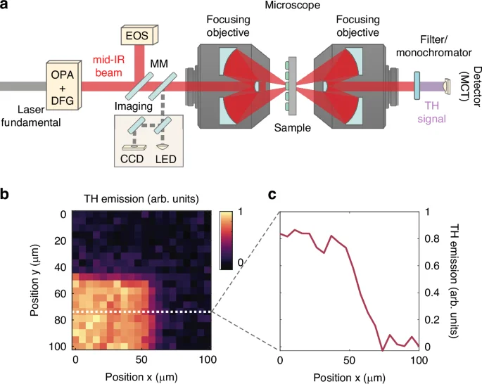
a Schematic representation of the experimental setup used for the THG experiment. The fundamental beam out of a Yb:KGW laser amplifier is used to drive a tunable mid-IR source, based on difference frequency generation (DFG) between a noncollinear optical parametric amplifier (OPA) and the laser fundamental. Using a mirror on a magnetic mount (MM) the generated mid-IR transients can be characterized by means of electro-optic sampling (EOS). The mid-IR pulses are coupled into the InGaAs nanoantennas through a reflective microscope and filtered after the interaction with the sample. The emitted third-harmonic signal is collected and measured by an MCT detector. b Map of third harmonic emission from one of the nanoantenna arrays used in this experiment. c Profile of third harmonic emission as the beam position is scanned across the array edge (dotted lines in b)
THG emission itself is confirmed by measuring a spectrum of the emitted radiation with a dispersive spectrometer (compare SI) while ensuring that other orders of nonlinearity (mainly second) are filtered out. The intensity of the THG allows to calculate the number of third harmonic photons NTH emitted per pulse by the antenna array as a function of pump peak power density (Fig. 3a–e). The coefficient of the cubic fits defines the nonlinear efficiency of the THG process ηTHG for each pair of λFF and n0 values. Above a certain threshold, we observe a deviation from the expected cubic behavior due to heating38 and/or free electron current saturation effects in high driving fields37, and the corresponding data points are omitted in the fitting. The values of λFF = 6.3 μm, 7.7 μm, 9.0 μm, 10.3 μm, and 12.0 μm are above, close to, or below λp = 9.62, 7.97, and 7.33 μm for the three samples. The undoped reference nanoantenna sample, which eliminates free-electrons contributions of nonlinearity, showed very weak THG for all λFF.
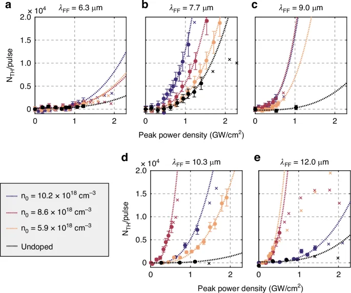
a–e Fluence dependence of the THG at different doping levels (color coded) and different fundamental field wavelengths λFF (different panels). A cubic fit model NTH = a + ηTHGx3 extracts the nonlinear coefficient, omitting data points (x) within a saturation regime
Discussion
To reveal the mechanism at the origin of the free-carrier-density dependent THG, we have numerically solved Eq. (1) together with the wave equation, following a perturbative approach using a finite-element method (see SI), with n0 and λFF as free parameters. Because of the rapid variations of the fields at the semiconductor surface introduced by the hydrodynamic terms, it is computationally very challenging to perform full three-dimensional (3D) calculations of the antenna system39. Here we used the two-dimensional (2D) equivalent model of Fig. 4a to simulate the single antenna. The 2D model reproduces the main linear spectral characteristics of the 3D system in Fig. 1d as long as a systematic shift of approximately Δλ ≃ −0.6 μm is taken into account (see SI). More importantly, the absorption spectra of the 3D antenna array align well with that of the 3D single antenna (SI), revealing a negligible inter-antenna coupling. This is due to the large gap between every two antennas. This fact validates our strategy of independent-antenna approximation with which the nonlinear coefficient could be scaled by the number of antennas involved when compared with experiments. The numerical nonlinear efficiencies of a single antenna are summarized in Fig. 4b–d, where we show color maps of the nonlinear coefficient ({eta }_{THG}=frac{{N}_{{rm{TH}}}}{{I}_{{rm{FF}}}^{3}}) as a function of λFF and n0, with NTH being the THG photon count per pulse and IFF the fundamental field power density in GW/cm2.
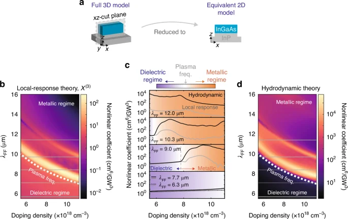
a Schematic of the equivalent 2D model. Maps of nonlinear coefficient of the single antenna with different fundamental field (FF) wavelengths and doping density based on (b), local model with only χ(3), or (d), nonlocal hydrodynamic model with both χ(3) and hydrodynamic sources. White dotted lines indicate the screened plasma wavelength on different doping densities which infers the condition Re(ε) = 0. The gray horizontal lines indicate the fundamental field wavelengths used in the experiments but with a 0.6 μm blueshift due to the correction between 2D and 3D models as discussed in the SI. (c) indicates the specific nonlinear coefficients under the experimental configurations based on the local-response (gray lines) or hydrodynamic (black lines) model. In the dielectric regime, theoretical results of λFF = 6.3 μm (dashed lines) are comparable with λFF = 7.7 μm. The colormap indicates different regimes
In Fig. 4b we considered a local-response theory with the dielectric susceptibility χ(3) as the only source of nonlinearity (Eq. (2a) where ({{bf{S}}}_{3omega }^{(3)}) is artificially set to zero). Single particle nonlinearities due to non-parabolicity are of the same order of dielectric nonlinearities in heavily doped semiconductors40, therefore much weaker than hydrodynamic nonlinearities as we show here. The plasmonic field enhancement of the nanoantennas is included in the calculation as a Drude term. In Fig. 4d both nonlinear contributions of Eq. 2 and (2b) were included (see also pure hydrodynamic contributions in SI). The strong dependence of ηTHG on n0 is markedly different at each λFF as we highlight in Fig. 4c, where we plot a few selected horizontal cuts of the color maps.
We can identify three different regimes: i) the dielectric regime, when λFF < λp, i.e., below the white dotted line in Fig. 4b, d and in the bottom panel (λFF = 6.3 and 7.7 μm) of Fig. 4c; ii) the plasmonic resonance regime, when λFF ≃ λLSPR, i. e., the bright regions just above the white dotted line in Fig. 4b, d and in the λFF = 9.0 and 10.3 μm panels in Fig. 4c); iii) the metallic regime when λFF > λp as in the upper parts of Fig. 4b, d and in the top panel (λFF = 12.0 μm) of Fig. 4c.
Considering the local response (gray curves in Fig. 4c) we observe an enhancement of ηTHG above the dielectric-χ(3) level of 101 cm6/ GW3 only in the plasmonic resonance regime (broad peaks at n0 ~ 7 × 1018 cm−3 for λFF = 10.3 μm and n0 ~ 9.5 × 1018 cm−3 for λFF = 9.0 μm). This is due to the increase of the linear extinction cross-section of the antennas at the LSPR, which effectively increases the polarization field within the material. The peak value of ηTHG is in the range 102 cm6/GW3, 20 times higher than the dielectric-χ(3) baseline level. In the metallic regime at λFF = 12.0 μm, ηTHG drops to zero for high n0, because there is very small field penetration in the material.
Considering the hydrodynamic case (black curves in Fig. 4c), ηTHG is generally much higher than in the local case, apart from the dielectric regime (violet background in Fig. 4c). In the plasmonic resonance regime, ηTHG shows a broad enhancement at similar n0 values as for the local theory, and the magnitude of the enhancement is 200 times stronger (in total, almost 5000 times stronger than the dielectric-χ(3) baseline level). This cannot be accounted for by the pump extinction enhancement, which affects both source terms equally, therefore it must be due to the hydrodynamic nonlinearity of Eq. (2b). Contrarily to the local-response theory, the nonlinear coefficient enhancement is still visible in the metallic regime, where plasmon fields at the semiconductor surface still exist even out of resonance: the very small field penetration in the bulk does not impact on the hydrodynamic nonlinearity, which originates close to the antenna surface, where gradients are strongest. For λFF = 12.0 μm, ηTHG is nonzero for high n0 and it is especially strong for decreasing n0, up to 104 cm6/GW3.
We now compare the experimental data with the numerical calculations performed with an “effective” decay γ = 3γ0 to account for the overall damping due to the imperfection that broadens the resonances as observed with linear optical characterization. To compare the numerical THG efficiency with the experimental one, we have estimated the beam width at full-width-half-maximum to be ~80 μm, which implies that ~640 antennas contributed to the measured THG.
The ηTHG retrieved from the cubic fits in Fig. 3a–e are summarized in Fig. 5a as a function of λFF. At high doping densities and long wavelengths λFF (metallic regime), Fig. 5a shows that the nonlinear coefficient predicted by hydrodynamic theory matches the experimental data, in stark contrast with the results of the local-response theory. In this regime, the nonlinear coefficients predicted by the hydrodynamic theory, proved by the experiments, have a two-orders of magnitude enhancement (~105 cm6/GW3) compared with the local-response model (~103 cm6/GW3). For the undoped case (lower panel of Fig. 5a), the two theories predict the same results due to the lack of free electrons and the absence of free-electron nonlinearity (dielectric regime). The theories predict low and spectrally flat optical nonlinearity, matching the experimental results.
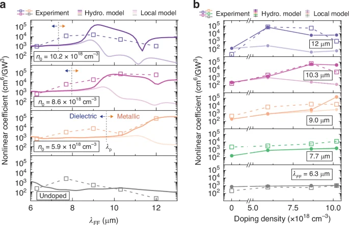
a Nonlinear coefficients as a function of the fundamental field wavelength λFF of different doping densities n0. Experimental data (markers with dashed lines) was compared with theoretical results from hydrodynamic theory (darker solid lines), and classical local-response model with only a dielectric χ(3) (lighter solid lines). Metallic and dielectric regimes are separated by a dashed line at plasma wavelength λp. b Nonlinear coefficients as a function of doping densities, excited with different λFF acquired from the experiments (markers), hydrodynamic theory (darker solid lines), and classical local-response model (lighter solid lines). Numerical data were obtained by properly normalizing 2D calculations and considering a broadened damping of 3γ0 (see SI)
Figure 5b represents the nonlinear THG coefficient as a function of doping density n0, to compare the experimental results with Fig. 4. At the shortest fundamental field wavelength λFF = 6 μm, the two theories overlap and predict low nonlinearity. In contrast, at the highest doping and long wavelength (metallic regime), the high THG coefficients can be explained only within the hydrodynamic theory. The three experimental conditions that have provided the highest ηTHG are λFF = 12.0 μm (blue squares) and n0 = 5.9 and 8.6 × 1018 cm−3, and λFF = 10.3 μm (violet squares) and n0 = 8.6 × 1018 cm−3. Remarkably the hydrodynamic model and the experimental nonlinear coefficients are of the same order of magnitude (~105 cm6/GW3). In summary, the experiment agrees well with the main hydrodynamic model predictions in Fig. 5, where efficiencies in the metallic regime (long λFF) are generally much higher than in the dielectric regime (short λFF), while the local-response model in Fig. 5f predicts exactly the opposite behavior.
Conclusion
The combination of theory and experiments allows us to demonstrate that the fundamental origin for THG in optical nanoantennas made of heavily doped semiconductors is the nonlinear collective behavior of free electrons, described within a hydrodynamic formalism, as opposed to the conventional dielectric nonlinearity due to crystal lattice anharmonicity and bound electrons. which is described by a local susceptibility χ(3) independent of the doping level. The experiments show that the efficiency of THG could be up to two orders of magnitude larger than the dielectric one in InGaAs.
We can thus speculate then that free electrons might also be the predominant source of nonlinearity in all possible plasmonic systems and therefore might be relevant to a wide range of nonlinear experiments that involve gold nanoantenna arrays41. In this context, shorter length scales, stronger fields and higher energy loss might require further developments even beyond the hydrodynamic description presented, with interesting perspective of understanding collective oscillations in free electron gasses22. In addition, the employed semiconductor material platform (InGaAs/InP) is currently under scrutiny to realize photonic integrated circuits in the mid-IR, featuring all-semiconductor waveguides and resonators17,18,19. Plasmonic effects, introduced by selectively doping specific volumes, could provide such photonic integrated circuits with tailored giant nonlinear coefficients. If realized, this new type of tunable nonlinear photonic circuit holds promise for nonlinear signal processing.
Finally, our study underscores the importance of a holistic approach in the design of optical nanoantennas. The local theory allows for the identification of the nonlinear source distribution with the local optical pump intensity patterns. Instead, to quantify the hydrodynamic nonlinearity the full equations of motion of the electron fluid in an external optical field must be solved for each specific geometry. In summary, the nonlocal hydrodynamic response adds a layer of complexity to nonlinear plasmonic device design, but it also unlocks a richer landscape of opportunities.
Materials and methods
Growth and antenna fabrication
The InGaAs thin films were grown by MOCVD (Metal Organic Chemical Vapor Deposition) on InP substrates. The films were doped with Si leading to a n-doping of the material. The thickness of the InGaAs film was about 3 μm. The doping levels of the thin films were calculated by measuring the reflectance by means of Fourier-transform infrared spectroscopy (FTIR) and by performing a Drude fit. The antenna arrays were fabricated by lithography and etching the InGaAs film, after thinning down the InGaAs epi-layer to 800 nm with wet chemical etching.
Linear characterization
The antenna arrays were investigated by micro-FTIR spectroscopy to measure their plasmonic resonances. The measurements were carried out with a commercial Bruker IFS-66V Michelson interferometer coupled to an infrared microscope (Hyperion). The objective was reflective cassegrain-type with a numerical aperture (NA) of 0.4 and a magnification of 15x. The detector is a liquid nitrogen-cooled Mercury Cadmium Telluride (MCT). The FTIR measurements of the antenna arrays were performed both in reflection (R) and in transmission (T), and the absorption coefficients shown in Fig 1d were calculated as 1−R−T.
Nonlinear characterization
Our tunable mid-IR source is based on a Yb:KGW laser amplifier, emitting 100 μJ pulses with 1030 nm central wavelength and operating at a repetition rate of 100 kHz. Fundamental wavelength (FW) pulses with energy of 50 μJ drive a noncollinear optical parametric amplifier (NOPA), delivering broadband near-infrared pulses tunable in the range between 1050 and 1400 nm and 1 μJ pulse energy. The output of the NOPA and the remaining 50 μJ of laser FW are collinearly focused onto a 1.2-mm-thick GaSe crystal, where p-polarized mid-IR pulses (with pulse energy up to 100 nJ) are generated by means of difference frequency generation (DFG) in a type-II configuration. The spectrum of the mid-IR pulses can be tuned by a suitable selection of the NOPA output central wavelength along with careful adjustments of the phase-matching conditions. The resulting mid-IR transients are characterized by means of electro-optic sampling, yielding for all the excitation pulses used in this work a temporal duration of 400 fs, a bandwidth of 1.5 THz and peak electric fields up to 10 MV/cm. The mid-IR pulses are coupled into the InGaAs antennas using a confocal microscope operating in transmission geometry and based on gold-coated dispersionless Cassegrain reflective objectives with 0.5 numerical aperture (NA).
The microscope can also be used in reflective geometry to image the sample and locate the antenna arrays. The emitted third harmonic radiation is measured using a liquid-nitrogen-cooled MCT detector and lock-in readout. In order to filter the fundamental mid-IR pulse from the third-harmonic emission, we have used a 5mm thick sapphire window, which acts as a short pass filter with transmission edge at 5 μm. In order to filter spurious second harmonic emission from the substrate we have employed either crystalline filters or a monochromator, depending on the excitation wavelength. The monochromator has also been used to record the spectrum of the third-harmonic emission from the antennas.
To calculate the number of TH photons from the voltage signal at the MCT detector, we used the following calibration procedure. We accounted for the wavelength sensitivity of the photovoltaic MCT detector and with the loss factors due to lenses and glass filters. When we performed measurements with the monochromator, we have also considered the spectral efficiency of the grating and the finite bandwidth of the monochromator output. We have corrected this by comparing the third harmonic signal both with the monochromator and using glass filters at the same wavelength. To transform the detector output voltage into a number of photons emitted, we have then measured the fundamental beam (at λFF=12.0μm) both with a thermal power meter and with the MCT detector. The power value is then converted into the number of photons N emitted per pulse using the relation P = Epulsef = Nphotonshνf where Epulse is the pulse energy, h is the Planck constant, ν the central frequency of third harmonic emission and f is the repetition rate of the laser.
Simulations
We used the finite-element method (COMSOL Multiphysics) to solve the differential equation system formed by the free-electrons equation and the electromagnetic wave equation in the frequency domain. The customized coupled equations were implemented using proper weak-form expressions. Overall, three steps, where each step solving for each harmonic (ω, 2ω, 3ω), were used to take both cascaded and direct THG into account, see details in SI.
Online content
Any methods, additional references, Nature Research reporting summaries, source data, extended data, supplementary information, acknowledgments, peer review information; details of author contributions and competing interests; and statements of data and code availability are available at https://doi.org/10.1038/s41377-025-01783-4.
Data availability
Source data are available for this paper. All other data that support the plots within this paper and other findings of this study are available from the corresponding author upon reasonable request.
Code availability
The COMSOL models are available from the corresponding author upon reasonable request.
References
-
Boyd, R. & Prato, D. Nonlinear Optics (Academic Press, 2008).
-
Brida, D., Krauss, G., Sell, A. & Leitenstorfer, A. Ultrabroadband Er: fiber lasers. Laser Photonics Rev. 8, 409–428 (2014).
Google Scholar
-
Liu, Y. et al. A photonic integrated circuit–based erbium-doped amplifier. Science 376, 1309–1313 (2022).
Google Scholar
-
Biagioni, P., Huang, J.-S. & Hecht, B. Nanoantennas for visible and infrared radiation. Rep. Prog. Phys. 75, 024402 (2012).
Google Scholar
-
Grinblat, G. Nonlinear dielectric nanoantennas and metasurfaces: frequency conversion and wavefront control. ACS Photonics 8, 3406–3432 (2021).
Google Scholar
-
Kauranen, M. & Zayats, A. V. Nonlinear plasmonics. Nat. Photonics 6, 737 – 748 (2012).
Google Scholar
-
Panoiu, N. C., Sha, W. E. I., Lei, D. Y. & Li, G.-C. Nonlinear optics in plasmonic nanostructures. J. Opt. 20, 083001 (2018).
Google Scholar
-
Krasavin, A. V., Ginzburg, P. & Zayats, A. V. Free-electron optical nonlinearities in plasmonic nanostructures: a review of the hydrodynamic description. Laser Photonics Rev. 12, 1700082 (2018).
Google Scholar
-
Pu, Y., Grange, R., Hsieh, C.-L. & Psaltis, D. Nonlinear optical properties of core-shell nanocavities for enhanced second-harmonic generation. Phys. Rev. Lett. 104, 207402 (2010).
Google Scholar
-
Lehr, D. et al. Enhancing second harmonic generation in gold nanoring resonators filled with lithium niobate. Nano Lett. 15, 1025–1030 (2015).
Google Scholar
-
Shibanuma, T., Grinblat, G., Albella, P. & Maier, S. A. Efficient third harmonic generation from metal-dielectric hybrid nanoantennas. Nano Lett. 17, 2647–2651 (2017).
Google Scholar
-
Kuzyk, M. G. Physical limits on electronic nonlinear molecular susceptibilities. Phys. Rev. Lett. 85, 1218 (2000).
Google Scholar
-
Ciracì, C. & Della Sala, F. Quantum hydrodynamic theory for plasmonics: Impact of the electron density tail. Phys. Rev. B 93, 205405 (2016).
Google Scholar
-
De Luca, F., Ortolani, M. & Ciracì, C. Free electron nonlinearities in heavily doped semiconductors plasmonics. Phys. Rev. B 103, 115305 (2021).
Google Scholar
-
De Luca, F. & Ciracì, C. Impact of surface charge depletion on the free electron nonlinear response of heavily doped semiconductors. Phys. Rev. Lett. 129, 123902 (2022).
Google Scholar
-
De Luca, F., Ortolani, M. & Ciracì, C. Free electron harmonic generation in heavily doped semiconductors: the role of the materials properties. EPJ Appl. Metamater. 9, 13 (2022).
Google Scholar
-
Jung, S. et al. Homogeneous photonic integration of mid-infrared quantum cascade lasers with low-loss passive waveguides on an InP platform. Optica 6, 1023 (2019).
Google Scholar
-
Kazakov, D. et al. Active mid-infrared ring resonators. Nat. Commun. 15, 607 (2024).
Google Scholar
-
Wang, R. et al. Monolithic integration of mid-infrared quantum cascade lasers and frequency combs with passive waveguides. ACS Photonics 9, 426–431 (2022).
Google Scholar
-
Scalora, M. et al. Electrodynamics of conductive oxides: Intensity-dependent anisotropy, reconstruction of the effective dielectric constant, and harmonic generation. Phys. Rev. A 101, 053828 (2020).
Google Scholar
-
Maack, J. R., Mortensen, N. A. & Wubs, M. Size-dependent nonlocal effects in plasmonic semiconductor particles. EPL (Europhys. Lett.) 119, 17003–8 (2017).
Google Scholar
-
Rodríguez-Suné, L. et al. Study of second and third harmonic generation from an indium tin oxide nanolayer: Influence of nonlocal effects and hot electrons. APL Photonics 5, 010801 (2020).
Google Scholar
-
Toscano, G. et al. Resonance shifts and spill-out effects in self-consistent hydrodynamic nanoplasmonics. Nat. Commun. 6, 7132 (2015).
Google Scholar
-
Yan, W. Hydrodynamic theory for quantum plasmonics: linear-response dynamics of the inhomogeneous electron gas. Phys. Rev. B 91, 115416 (2015).
Google Scholar
-
Ceglia, D. D. et al. Viscoelastic optical nonlocality of low-loss epsilon-near-zero nanofilms. Sci. Rep. 8, 874 (2018).
Google Scholar
-
Raza, S., Bozhevolnyi, S. I., Wubs, M. & Mortensen, N. A. Nonlocal optical response in metallic nanostructures. J. Phys.: Condens. Matter 27, 183204 (2015).
Google Scholar
-
Ciracì, C. Current-dependent potential for nonlocal absorption in quantum hydrodynamic theory. Phys. Rev. B 95, 245434 (2017).
Google Scholar
-
Manfredi, G. How to model quantum plasmas. Fields Inst. Commun. 46, 263–287 (2005).
Google Scholar
-
Dias, E. J. C. et al. Probing nonlocal effects in metals with graphene plasmons. Phys. Rev. B 97, 245405 (2018).
Google Scholar
-
Pellegrini, G. et al. Benchmarking the use of heavily doped ge for plasmonics and sensing in the mid-infrared. ACS Photonics 5, 3601–3607 (2018).
Google Scholar
-
Taliercio, T. & Biagioni, P. Semiconductor infrared plasmonics. Nanophotonics 8, 949 – 990 (2019).
Google Scholar
-
Frigerio, J. et al. Tunability of the dielectric function of heavily doped germanium thin films for mid-infrared plasmonics. Phys. Rev. B 94, 085202 (2016).
Google Scholar
-
Fischer, M. P. et al. Optical activation of germanium plasmonic antennas in the mid-infrared. Phys. Rev. Lett. 117, 047401 (2016).
Google Scholar
-
Troha, T. et al. Ultrafast long-distance electron-hole plasma expansion in GaAs mediated by stimulated emission and reabsorption of photons. Phys. Rev. Lett. 130, 226301 (2023).
Google Scholar
-
Zhang, S., Bao, K., Halas, N. J., Xu, H. & Nordlander, P. Substrate-induced fano resonances of a plasmonic nanocube: a route to increased-sensitivity localized surface plasmon resonance sensors revealed. Nano Lett. 11, 1657–1663 (2011).
Google Scholar
-
Baldassarre, L. et al. Midinfrared plasmon-enhanced spectroscopy with germanium antennas on silicon substrates. Nano Lett. 15, 7225–7231 (2015).
Google Scholar
-
Fischer, M. P. et al. Plasmonic mid-infrared third harmonic generation in germanium nanoantennas. Light Sci. Appl. 7, 106 (2018).
Google Scholar
-
Lang, D. et al. Nonlinear plasmonic response of doped nanowires observed by infrared nanospectroscopy. Nanotechnology 30, 084003 (2018).
Google Scholar
-
Vidal-Codina, F., Nguyen, N.-C., Ciracì, C., Oh, S.-H. & Peraire, J. A nested hybridizable discontinuous Galerkin method for computing second-harmonic generation in three-dimensional metallic nanostructures. J. Comput. Phys. 429, 110000 (2021).
Google Scholar
-
Khurgin, J. B., Clerici, M. & Kinsey, N. Fast and slow nonlinearities in epsilon near zero materials. Laser Photonics Rev. 15, 2000291 (2021).
Google Scholar
-
Celebrano, M. et al. Evidence of cascaded third-harmonic generation in noncentrosymmetric gold nanoantennas. Nano Lett. 19, 7013–7020 (2019).
Google Scholar
Acknowledgements
D.B., A.R., and T.D. acknowledge funding by the European Research Council (819871) and the European Regional Development Fund (2017-03-022-19). S.M. acknowledges the Lee-Lucas Chair in Physics. A.T. and E.B. acknowledge funding by the Deutsche Forschungsgemeinschaft (DFG, German Research Foundation) under grant numbers EXC 2089/1-390776260 (Germany’s Excellence Strategy) and TI 1063/1 (Emmy Noether Program), by the European Research Council (METANEXT, 101078018), and the Center for NanoScience (CeNS). A.B. and R.C. acknowledge financial support from the French National Research Agency: project BIRD (Project ANR-21-CE24-0013). H.H., T.V., A.B., V.G., M.P., I.S., G.B., E.B., A.T., R.C., M.O., and C.C. acknowledge funding from the European Union under the European Innovation Council (EIC) project NEHO (Grant No.101046329). Views and opinions expressed are those of the authors only and do not necessarily reflect those of the European Union or the European Innovation Council and SMEs Executive Agency (EISMEA). Neither the European Union nor the granting authority can be held responsible for them. This work is partly supported by the RENATECH network and the General Council of Essonne.
Author information
Authors and Affiliations
Contributions
A. Rossetti: experimental investigation and methodology (nonlinear characterization), data curation, review, and editing. H. Hu: numerical investigation and theoretical methodology, data curation, review, and editing. T. Venanzi: experimental investigation and methodology (optical characterization), data curation, review and editing. A. Bousseksou: fabrication, and experimental investigation and methodology (morphology characterization). F. De Luca: formal analysis, theoretical methodology, review and editing. T. Deckert: experimental investigation and methodology (nonlinear characterization), review and editing. V. Giliberti: experimental methodology (optical characterization), review and editing. M. Pea: experimental methodology, review, and editing. I. Sagnes: semiconductor epitaxy, review and editing. G. Beaudoin: semiconductor epitaxy, review, and editing. P. Biagioni: formal analysis, review, and editing. E. Baù: formal analysis, review, and editing. S. Maier: formal analysis, review and editing. A. Tittl: formal analysis, review, and editing. D. Brida: experimental methodology (nonlinear characterization), formal analysis, review, and editing. R. Colombelli: fabrication methodology, formal analysis, review and editing. M. Ortolani: conceptualization, formal analysis, writing of the original draft, review, and editing. C. Ciracì: conceptualization, formal analysis, theoretical methodology, writing of the original draft, review, and editing.
Corresponding authors
Ethics declarations
Conflict of interest
The authors declare no competing interests.
Supplementary information
Control and enhancement of optical nonlinearities in plasmonic semiconductor nanostructures
Rights and permissions
Open Access This article is licensed under a Creative Commons Attribution 4.0 International License, which permits use, sharing, adaptation, distribution and reproduction in any medium or format, as long as you give appropriate credit to the original author(s) and the source, provide a link to the Creative Commons licence, and indicate if changes were made. The images or other third party material in this article are included in the article’s Creative Commons licence, unless indicated otherwise in a credit line to the material. If material is not included in the article’s Creative Commons licence and your intended use is not permitted by statutory regulation or exceeds the permitted use, you will need to obtain permission directly from the copyright holder. To view a copy of this licence, visit http://creativecommons.org/licenses/by/4.0/.
Reprints and permissions
About this article
Cite this article
Rossetti, A., Hu, H., Venanzi, T. et al. Control and enhancement of optical nonlinearities in plasmonic semiconductor nanostructures.
Light Sci Appl 14, 192 (2025). https://doi.org/10.1038/s41377-025-01783-4
-
Received: 20 August 2024
-
Revised: 21 January 2025
-
Accepted: 09 February 2025
-
Published: 13 May 2025
-
DOI: https://doi.org/10.1038/s41377-025-01783-4