
Abstract
Political responses to the COVID-19 pandemic led to changes in city soundscapes around the globe. From March to October 2020, a consortium of 261 contributors from 35 countries brought together by the Silent Cities project built a unique soundscape recordings collection to report on local acoustic changes in urban areas. We present this collection here, along with metadata including observational descriptions of the local areas from the contributors, open-source environmental data, open-source confinement levels and calculation of acoustic descriptors. We performed a technical validation of the dataset using statistical models run on a subset of manually annotated soundscapes. Results confirmed the large-scale usability of ecoacoustic indices and automatic sound event recognition in the Silent Cities soundscape collection. We expect this dataset to be useful for research in the multidisciplinary field of environmental sciences.
Research on key acoustic characteristics of soundscapes of the classical Chinese gardens
Acoustic Characterization of Edzna: A Measurement Dataset
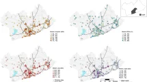
Space-time characterization of community noise and sound sources in Accra, Ghana
Background & Summary
In response to the rapid spread of the coronavirus disease 2019 (COVID-19) around the world, governments of many countries adopted physical distancing measures in early 2020, including more or less drastically restricting individual travel and suspending many work and leisure activities deemed ‘non-essential’1,2,3. Incidentally, these public health policy decisions opened a window of opportunity for many environmental scientists to investigate the effects of such a reduction in human activity on ecosystems at multiple spatiotemporal scales4,5,6,7,8.
The modification of soundscapes, especially in urban and peri-urban areas, was among the most significant environmental changes observed during this period9,10,11,12,13,14. The sudden decrease in individual travel and motorized transport of people and goods shaped extraordinary soundscapes in most cities of the world for a few weeks. This revealed the richness of animal sounds in urban areas, previously hidden by a multitude of anthropogenic sounds. Such a change, directly perceptible by the population, even raised interest outside the academic sphere, as reflected in numerous articles in the general press. Among the thousands of press articles on the subject, we will particularly mention the interactive publications produced by The New York Times (see, for example: The Coronavirus Quieted City Noise. Listen to What’s Left; or: The New York City of Our Imagination).
From an academic point of view, several studies have already been carried out on these “soundscapes of a confined world”, at different scales and in different types of spaces and territories (sub-continents15, countries16,17,18,19,20,21, regions22,23,24,25, cities18,26,27,28,29,30,31,32,33, neighborhoods29,34, protected natural areas35, semi-anthropized environments36,37,38, tourist sites39). Among these studies, some benefited from sensor networks predating the COVID-19 crisis, mobilizing for example underwater acoustics and/or seismic monitoring networks16,22,40, permanent noise pollution monitoring networks in urban environments26,41,42, or devices installed for pre-existing research projects43. Beyond these physical measurement approaches, several studies have also investigated individual and subjective perceptions of changes in soundscape composition. More specifically, the perceived proportion between natural and anthropogenic events in the soundscape is regularly raised in investigations that more broadly address the changes induced by different periods of population containment on experiential relationships to nature21,29,44.
In this paper, we present a global acoustic dataset45, collected between March and October 2020 by 261 contributors, at 317 sites distributed in 35 countries (Fig. 1). Recordings were primarily collected using Open Acoustic Devices AudioMoth46 or Wildlife Acoustics Song Meters SM4 (www.wildlifeacoustics.com) programmable recorders, which are widely used within the professional and amateur naturalist communities. This dataset is unique, with its international dimension, collaborative construction and open access availability. The acoustic data are presented in addition to climate classification and surrounding environment, offering a more comprehensive understanding of their significance and implications. In addition, we provide a set of descriptors based on ecoacoustic indices47 and on automatic recognition of sound categories using a pretrained deep neural network48. These descriptors were subsequently validated by collecting expert annotations on a small subset of the dataset, with which we derived statistical models to demonstrate their usability.
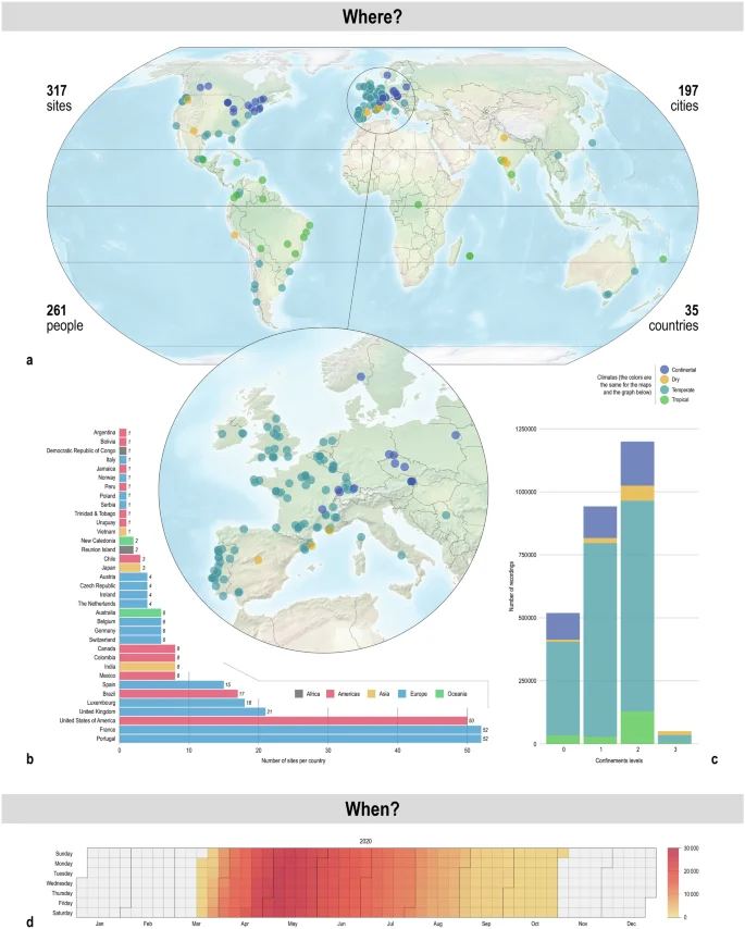
Panel a. Global and European mapping of recording sites. Colors refer to climates. Panel b. Number of recording sites per country. Colors refer to continents. Panel c. Number of recordings by confinement level and climate. Panel d: temporal distribution of global sampling effort, in number of recordings.
Methods
Silent Cities is a data collection that involved programmable audio recordings worldwide. The global scale of the project warranted us to not only gather acoustical recordings, but also contextualize them. We first describe the data collection procedures, the contributors’ network and contextual information related to the recording sites, such as location, urban density, climate classification or governmental policies related to human population containment in response to COVID-19. Next, we describe the processing of acoustic measurements computed on all recordings, including ecoacoustic indices, automatic sound event recognition, and voice activity detection.
Data collection
Recording protocol
On March 16, 2020, the French government announced the upcoming first containment of the population. A few days later, a first version of the Silent Cities protocol was submitted to professional networks. Feedback from researchers but also from journalists, artists and biological conservation practitioners interested in contributing were received. As requested, a more inclusive version, opening up the possibility of using different equipment and sampling efforts while preserving requirements for further robust statistical analyses was proposed (https://osf.io/m4vnw/). This second and final version of the protocol was shared on March 25, 2020 and is described below.
Each contributor provided recording equipment. To homogenize the recordings collection, recording devices were configured to obtain a 1 minute-long recording every 10 minutes on a daily cycle schedule, with a sampling rate set at 48 kHz. All recorders were to be set in Coordinated Universal Time (UTC+00) with an output format in .wav. In order to have comparable data, the use of an audible SM4 (Wildlife Acoustics) or an AudioMoth (Open Acoustic Devices), which were the two most popular programmable recorders at the time, was recommended. However, any device with high quality recording, allowing the recording configuration requested, was accepted. To anticipate the return of high levels of anthropogenic sounds after the end of containment measures, the gain was to be set at “low” for the Audiomoth and at 31 dB for the SM4 (gain at 5 dB and preamplification at 26 dB). The final dataset includes 216 sites monitored by an Audiomoth, 47 by an SM4 and 54 by another device.
The sampling duration of the collection was locally dependent. The protocol recommended to continue recording a minimum of two weeks after the end of the total city shut down and restoration of “normal” activities. However, the expected scenario of the return to “normal” activity extended well beyond predictions as the magnitude of the pandemic became progressively realised. As containment measures were being lifted in many countries during the summer, the acoustic sampling was ended on July 31, allowing contributors to continue collecting data after this date based on local situations. To summarise, the entire recordings collection covers the period from March 16 to October 31, 2020, with the highest number of recordings between April and July (see Fig. 1d).
Originally, contributors were able to choose between three levels of sampling effort based on their ability to record during the entire or partial duration of the project. Hereafter, we refine the definition of those levels to better fit the diversity of recording profiles represented in the final data set:
-
expert – The daily cycle schedule, duration of files and sampling rate were set according to the recommendations, and the duration of the sampling period was at least two months;
-
modified – The parameters are set as recommended but the sampling period is less than two months or some parameters such as the file duration, the sampling rate or the daily cycle schedule are different (i.e. every 3 hours), while conserving a fixed recording pattern along the sampling period;
-
opportunistic – All other sites that do not show any type of recording patterns.
The expert protocol was applied by 228 contributors, while the modified protocol and the opportunistic protocol were followed respectively by 72 and 17 contributors.
International contributor network
The dataset45 results from the collaborative work of 261 international contributors from various professional fields: 182 are academics, 37 are conservationist practitioners, 12 are artists and 30 do not recognize themselves in the three previous groups. An Open Science Foundation (OSF) project45 was created to organize the data collection and guarantee its open access with no restrictions. Other tools used to manage the collaborative work were Framaforms (https://framaforms.org/abc/fr/) to collect metadata about sites and contributors from the consortium.
Site descriptions
The containment of a large number of citizens worldwide restricted the location of the recorders. Contributors deployed their recorder on private land or a balcony at their residency (example on Fig. 2a). We encouraged those living in (peri-)urban areas to participate, even though recordings were also collected in rural areas. The soundscape recordings were collected from 317 sites located in or around 197 cities and 35 countries (see Fig. 1). In order to protect citizens’ privacy, the exact coordinates of the sites remain unknown and the location of the sites were based on the coordinates of their corresponding cities and approximate neighborhood. The sites cover four of the five climates defined by the Köppen climate classification49, with a majority of sites located in the temperate and dry climates and a spatial sampling in favor of the European and American continents (see Fig. 1). For each site, we extracted information about the surrounding land cover (more specifically the percentage of built-up and tree cover within a 1 km radius buffer scale around the sites; 100 m resolution50), human footprint (from 0 to 50, with the lowest score depicting the least human influence, 1 km resolution51,52), and population density (no. of inhabitants per square kilometer, 1 km resolution53) to document the degree of urbanization and human impact on the landscapes encompassing the recordings. In addition, contributors described in a few sentences the surroundings/context of their site. Thanks to the open data available on https://aa.usno.navy.mil/data/AltAz, we also extracted for each recording site the altazimuth coordinates of the Moon and Sun as well as the moon phase for each 10-second time interval during the days where soundscapes were collected. These data would be important for potential analysis about temporal soundscape dynamics. Finally, containment measures3 per country and date, summarized by the University of Oxford in the Oxford COVID-19 Government Response Tracker dataset, were downloaded from the web portal https://ourworldindata.org/grapher/stay-at-home-covid. These stay-at-home requirements are organized in 4 levels:
-
0 – No measures;
-
1 – Recommended not to leave home;
-
2 – Not allowed to leave home, with exceptions for daily exercise, grocery shopping, and other activities considered as essential;
-
3 – Not allowed to leave home, with rare exceptions (e.g. allowed to leave only once every few days, or only one person at a time).
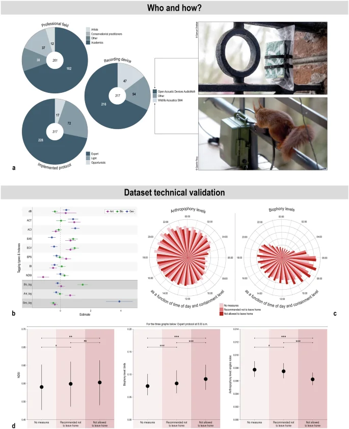
Panel a. Top left: Professional fields of the 261 participants. Middle: Distribution of type of devices for the 317 recording sites. Bottom left: type of protocol implemented. Right: Photos of the two main recording devices used: Open Acoustic Devices AudioMoth (top) and Wildlife Acoustics SM4 (bottom). Panel b. Association between the measured acoustic indices and tagging types and the presence of geophonical (Geo), biophonical (Bio) and anthropophonical (Ant) events detected manually by the contributors. Model estimates and associated 95% confidence intervals are represented with points and bars, respectively. Positive and negative estimates with confidence intervals not overlapping zero indicate positive and negative associations, respectively. Panel c. Radial barplots depicting the mean anthropophony and biophony level values per site, combining all protocols, recorded hourly throughout each period of COVID-19 containment levels. Panel d. Model predictions and associated 95% confidence intervals for NDSI, biophony (birds) and anthropophony (engine noise) levels at 8:00 a.m. during the COVID-19 confinement measures, following the expert protocol only. ***p < 0.001, **p < 0.010, *p < 0.050, ns: p > 0.050.
Due to the limited data collected during the strictest containment period (level 3, see Fig. 1c), we combined data from the two periods when leaving home was not permitted (levels 2 and 3) when performing the technical validation.
Acoustic measurements
All computations described here were performed with open-source packages or code from github, including scikit-maad (v1.4)54,55, librosa56 and pytorch57. The analysis code used to prepare this dataset is available for reference at https://github.com/brain-bzh/SilentCities.
Preprocessing audio
Audio preprocessing was divided into two steps. First, the file name, sample rate, date and relative sound pressure level were extracted from each audio recording. Then, each file (n = 2,701,378) was divided into 10-second segments (n = 16,252,373) in order to have a meaningful duration for both acoustic index calculation and automatic sound event recognition. The sampling rate of audio segments were homogenised at 48 kHz for acoustic index calculation and resampled to 32 kHz for automatic sound event recognition. For acoustic indices, the signals were filtered using a bandpass filter from 100 Hz to 20 kHz to remove low frequency electronic noise inherent to some recorders.
Acoustic Indices calculation
Acoustic diversity indices aim to summarize the overall complexity of an acoustic recording in a single mathematical value. Numerous acoustic indices have been previously proposed47,58,59, considering the time, frequency and/or amplitude dimensions of the recorded sound wave. We selected and calculated eight indices on all recordings; these indices were chosen based on their complementary and/or wide representation in the literature:
-
dB represents the relative acoustic energy of a signal;
-
dB Full Scale or dBfs represents the acoustic energy of a signal where the RMS value of a full-scale sine wave is defined as 0 dBfs60;
-
Acoustic Complexity Index or ACI61 measures the frequency modulation over the time course of the recordings. The value is calculated on a spectrogram (amplitude per frequency per time). ACI is described to be sensitive to highly modulated sounds, such as song birds, and less affected by constant sounds, such as background noise;
-
Activity or ACT62 corresponds to the fraction of values in the noise-reduced decibel envelope that exceed the threshold of 12 dB above the noise level. This noise level was estimated for each site by seeking the audio file yielding the minimum dB value;
-
Bioacoustic index or BI63 measures the area under the frequency spectrum (amplitude per frequency) above a threshold defined as the minimum amplitude value of the spectrum. This threshold represents the limit between what can be considered acoustic activity (above threshold) and what could be considered background noise (under threshold);
-
Entropy of the Average Spectrum or EAS62 is a measure of the ‘concentration’ of mean energy within the mid-band of the mean-energy spectrum;
-
Entropy of the Spectrum of Coefficients of Variation or ECV62 is derived in a similar manner to EAS except that the spectrum is composed of coefficients of variation, defined as variance divided by the mean of the energy values in each frequency bin;
-
Entropy of the Spectral Peaks or EPS62 is defined as a measure of the evenness or ‘flatness’ of the maximum-frequency spectrum, maximal frequencies being measured along the time of the recording. A recording with no acoustic activity should show a low EPS value, as all spectral maxima are low and constant over time;
-
Normalized Difference Soundscape Index or NDSI64 measures a ratio between biophony and anthropophony. The value of this index is calculated on a spectrogram and varies between -1, meaning the entire acoustic energy of the recording is concentrated under the frequency threshold of 2kHz and attributed to anthropophony only, and +1, meaning the entire acoustic energy of the recording is concentrated above the frequency threshold and attributed to biophony only.
Manual soundscapes description
In order to have a more thorough description of the recorded soundscapes, some contributors manually performed sound identification on a subset of their recordings. Two non-consecutive days of recordings were randomly selected for each site and each one-minute-long audio file recorded at the beginning of each hour was analysed (i.e. a total of 48 1-min files). Using software dedicated to sound analysis (e.g. Audacity: https://www.audacityteam.org/, Sonic visualizer: https://www.sonicvisualiser.org/, and Kaleidoscope: https://www.wildlifeacoustics.com/uploads/user-guides/Kaleidoscope-User-Guide.pdf), contributors were to (i) listen and view spectrograms of the recordings, (ii) estimate the percentage of time occurence (0%, 1-25%, 25-50%, 50-75% and 75-100%) of geophonic, biophonic, and anthropophonic events in each audio file, and (iii) provide more information about the source/type (e.g. geophony: wind, rain and river; biophony: birds, mammals and insects; anthropophony: car, plane and music) of each event. They further indicated the strength/intensity (on a scale from 0 to 3) of the identified geophonic and anthropophonic events and to provide for each biophonic event the number of different song/call/stridulation types visible on the spectrogram. Scoring per recording was associated with a confidence level on a scale from 1 to 5 (see Table 3 for an example of the identification table, inspired from protocol proposed in65).
A total of 1351 minutes of sounds were manually described from 30 sites. Contributors from Europe (Austria, Czech Republic, France, Germany, Ireland, Poland, Portugal, Serbia, and United Kingdom), the Americas (Canada, Colombia, Mexico, and United States of America), and Australia participated in the manual sound identification process. The number of audio files described varied slightly between participants (min: 9 minutes, max: 96, median: 48, mean: 45). Most audio files manually analyzed were recorded using AudioMoth (19 sites) and SM4 (8 sites).
Recordings were dominated by geophonic, biophonic and anthropophonic events (i.e. time occurence >75% within 1-min files) in 20, 34 and 51% of the 1351 minutes of sounds recorded, respectively. The most detected geophonic sounds were from wind (26% of the total number of records, including 76 records with strong wind intensity) and rain (12%). Bird calls (63%) and insect stridulations (16%) were the most encountered biophonic sounds. Around one third of the recordings with bird calls contained at least four different bird call types. Noise from cars (61%) and people talking (26%) were responsible for most of the anthropophonic sounds.
Automatic sound event recognition
Automatic sound event recognition (SER) became an essential task due to the immense volume (around 20 Terabytes) of the Silent Cities dataset. We adopted the AudioSet ontology and dataset66, which covers a wide range of everyday sounds. We explored the viability of utilizing PANNs (pretrained audio neural networks) pretrained on the full AudioSet data (available online: https://github.com/qiuqiangkong/audioset_tagging_cnn). The choice of a pretrained model was driven by its generality, as it has been exposed to a wide range of sounds, rendering it suitable for recognizing various audio events. In implementing our methodology, we employ a zero-shot inference approach. This involves applying the pretrained model directly to the entirety of the Silent Cities recordings without the need for additional training or fine-tuning. By doing so, we can benefit from the model’s generalization capabilities and avoid the time-consuming process of manual annotation. To categorize the diverse audio events within our dataset, we leverage the Audioset ontology and make necessary adaptations. Specifically, we classify the sounds into three main types: anthropophony (sounds produced by human activities), biophony (sounds originating from natural living organisms), and geophony (sounds resulting from non-living sources like weather or geological activities). The details of sound event grouping (i.e. audio tagging types) and corresponding labels are presented in Table 4 to provide clarity and consistency in the classification process. This grouping was also done to have the same categories than in the manual annotation described in the previous section.
Voice activity detection
As many recordings in Silent Cities were performed at home (e.g. on a balcony) during periods of containment, human voices are likely to be heard and speakers may be easily identified. In order to prevent issues related to privacy, we identified audio segments containing speech and only shared in open access the audio segments without speech. Voice activity detection was conducted using a general purpose voice activity detector (GP-VAD) that was pretrained on noisy, natural speech recordings in the wild67 (available online: https://github.com/RicherMans/GPV). We applied GP-VAD on a subset of 250000 one-minute recordings (approx. 24 weeks). Detections on this subset were considered as a ground truth speech label, that we set a reference to detect speech in the entirety of the Silent Cities dataset, for which we have a weak speech label from the Audioset SER (described in the previous paragraph). More precisely, we used the GP-VAD predictions on the subset to estimate a receiver-operator characteristic curve, and by setting a true positive rate of detecting 75 % of speech recordings, we obtain an average false positive rate of 34 % false alarms when using the Audioset SER. The corresponding threshold was applied on the raw probability from the Audioset SER on the entirety of the dataset, which eventually resulted in a rejection of 2,868,098 10-second audio segments, representing approximately 18 % of the dataset.
Data Records
The dataset45 comprises the entire collection of acoustic recordings in Free Lossless Audio Codec (FLAC) format and associated metadata spread across several Comma Separated Value (CSV) tables (see Table 1). In order to protect privacy, only the preprocessed 10-second audio files with no speech identified are in direct open access on the OSF website (https://doi.org/10.17605/OSF.IO/H285U).
Technical Validation
To validate the Silent Cities dataset45, we verified the veracity of the metadata reported by the contributors and consolidated the acoustic recordings collections by checking for device malfunctions. We also verified whether the automated acoustic measurements conducted on the recordings were coherent with aural human observations. Finally, proof of validity of the dataset to reflect urban soundscape changes due to stay-at-home requirements is presented. The three steps of this technical validation are detailed below.
First, we verified the quality of the data by manually verifying that the recordings were correctly attributed to their dedicated site with the help of the contributors. We also ran a manual cleaning of information given by the contributors to remove any personal information, such as address or GPS coordinates, and to correct spelling mistakes to ensure interoperability between tables. In addition, we verified the conformity of the protocol by automatically extracting information from the recording collection (i.e. frequency range, schedule of recordings) and reported observed modification of the protocol. We also automatically and manually verified the proper calculation of acoustic measurements and identified 10,724 files for which the calculation failed, probably due to file-related issues; these files were excluded from the dataset without affecting an entire site (i.e. no sites were excluded because of this issue). Finally, we checked for recorder device malfunction by making sure of a temporal variation of the dB value for each recorder, only one site was identified with a flat dB response, leading to its exclusion from the dataset.
Second, we confirmed that the automated soundscape measurements informed and aligned with real soundscape events. More specifically, we investigated whether the acoustic indices and audio tagging categories were representative of geophonic, biophonic and anthropophonic events detected manually by the contributors. To do so, we conducted a series of univariate generalized linear mixed-effect models (GLMMs; ‘glmmTMB’ package68,) in R v4.2.1. We tested independently the presence/absence of geophonic, biophonic and anthropophonic events within the 1351 1-min recordings (i.e. response variables) in relation to acoustic indices and tagging types (i.e. explanatory variables). Models were fitted with a binomial error distribution and a logit link function. We considered the identity of contributors as a random effect to avoid pseudoreplication. We also implemented a first-order autoregressive function to account for serial autocorrelation in residuals. Statistical assumptions were visually assessed using model diagnostics (i.e. Quantile-Quantile plot, residuals vs fitted plot) with the DHARMa package69. The acoustic indices were linked to geophonic, biophonic, or anthropophonic events, albeit to varying degrees (Fig. 2b). For instance, the presence of biophonic events was associated with greater values of EAS and ECV and lower values of dB. Audio tagging categories effectively captured the intended soundscapes they aimed to portray (Fig. 2b).
Third, we assessed the validity of the dataset in evaluating the impact of stay-at-home requirements on soundscapes. In a first step, we plotted the mean values of biophony and anthropophony levels (here defined as the maximum probability of having a biophonic and anthropophonic event in the 1-min recording, respectively) per site recorded at each hour (all protocols combined). As expected, we observed temporal patterns in biophony and anthropophony levels throughout the day (Fig. 2c). Regardless of the time of day, biophony levels were greater during the period when leaving home was not permitted (i.e. confinement level 2 or 3) compared to the other periods, while the opposite pattern was true for anthropophony. In a second step, we modeled changes in the values of acoustic indices as well as biophony and anthropophony levels (i.e. response variables) in relation to the containment measures (i.e. explanatory variables) using GLMMs with a beta distribution and a log link function. We aimed to provide a proof of validity and therefore limited the analysis to the expert protocol and all recordings collected at 8:00 am (i.e. peak of biophonic and anthropophonic events; Fig. 2d). We focused on NDSI for the acoustic index and the probability of bird calls and engine noise indicated by the automatic sound event recognition in the recordings as proxies of biophony and anthropophony levels, respectively. We added as covariates in the models: (i) Julian day to consider seasonal changes in biological and anthropogenical sounds, (ii) the first Principal Component Analysis axis depicting the level of anthropization in the landscape surrounding the recordings, and (iii) the climate type. Continuous covariates were scaled (mean = 0; SD = 1) to avoid convergence issues. We considered as random effects site identity nested within country to account for hierarchical clustering within data and recorder type, due to potential sensitivity differences between devices. Due to the limited data collected during the strictest containment period, we combined data from the two periods when leaving home was not permitted. The same approach as outlined previously was employed for model validation (note that the validity of the statistical assumptions, assessed using Quantile-Quantile and residuals vs fitted plots, was only partially met for the engine noise model). Full models were more informative than the null ones with differences in Akaike Information Criterion scores > 500. Finally, we conducted Tukey’s post hoc multiple comparison test to investigate pairwise differences in NDSI values and biophony and anthropophony levels between the three COVID-19 containment measures investigated. Overall, we found that COVID-19 lockdown had positive effects on NDSI values and biophony levels and negative effects on anthropophony levels. After accounting for seasonal and landscape effects, our models suggest that NDSI values and biophony levels were significantly greater during the periods when leaving home was not recommended or permitted, compared to the period with no measures (Fig. 2d; Table 2). There were also higher biophony levels during the period when leaving home was not permitted than during the period with when leaving home was not recommended. The opposite patterns were found for the anthropophony levels, with significantly lower values measured during the periods when leaving home was not permitted compared to the other periods, albeit the differences were of smaller magnitude (Fig. 2d; Table 5). Altogether, our preliminary analysis revealed potential changes in soundscape patterns that can be attributed to containment policies, these changes being above expected differences due to climate.
Usage Notes
The Silent Cities dataset could be considered for multiple applications. In the specific fields of bio/ecoacoustics, it could be used to study the effect of containment measures on urban soundscapes29, to improve the performance of acoustic indices in urban environments70 and to gain a deeper understanding of the interplay between biophony and urban environment characteristics71. In the field of machine learning (machine listening, deep learning), it will allow the testing of difficult cases of generalization in sound event recognition from one site to another, due to the variety of sampled sites72. In the interdisciplinary field of territorial sciences (e.g. economic geography, territorial economics, spatial planning, urban engineering sciences), it will make it possible to analyze the links between the levels of economic activity of a city and the levels of noise pollution. Finally, for environmental sciences interested in well-being and relationships between humans and non-humans within urban socio-ecosystems (e.g. environmental and health psychology, landscape design, environmental geography, etc.), this dataset opens up opportunities for the qualitative study of individual and subjective perceptions of the different soundscape configurations collected. More broadly, we aim for this international and collaborative dataset to be usefully mobilized in any research working to make better coexistence between humans and non-humans possible, and thus working to maintain the Earth’s habitability conditions for all of them.
The Silent Cities dataset45 is available under the terms of a Creative Commons Attribution 4.0 International waiver (CC-BY 4.0, https://creativecommons.org/licenses/by/4.0/). The CC-BY-4.0 waiver facilitates the discovery, re-use, and citation of the dataset. When using all or part of the dataset, we require anyone to cite both the dataset45 and this publication.
Code availability
The recording manipulation and acoustic measurements were run using Python, https://github.com/brain-bzh/SilentCities and the analyses were run on R https://github.com/agasc/SilentCities-R.
References
-
Desvars-Larrive, A. et al. A structured open dataset of government interventions in response to covid-19. Scientific data 7, 285 (2020).
Google Scholar
-
Porcher, S. Response2covid19, a dataset of governments’ responses to covid-19 all around the world. Scientific data 7, 423 (2020).
Google Scholar
-
Hale, T. et al. A global panel database of pandemic policies (oxford covid-19 government response tracker). Nature human behaviour 5, 529–538 (2021).
Google Scholar
-
Gaiser, E. E. et al. Long-term ecological research and the covid-19 anthropause: A window to understanding social–ecological disturbance. Ecosphere 13, e4019 (2022).
Google Scholar
-
Rutz, C. et al. Covid-19 lockdown allows researchers to quantify the effects of human activity on wildlife. Nature Ecology & Evolution 4, 1156–1159 (2020).
Google Scholar
-
Bates, A. E., Primack, R. B., Moraga, P. & Duarte, C. M. Covid-19 pandemic and associated lockdown as a “global human confinement experiment” to investigate biodiversity conservation. Biological conservation 248, 108665 (2020).
Google Scholar
-
Diffenbaugh, N. S. et al. The covid-19 lockdowns: a window into the earth system. Nature Reviews Earth & Environment 1, 470–481 (2020).
Google Scholar
-
Warrington, M. H., Schrimpf, M. B., Des Brisay, P., Taylor, M. E. & Koper, N. Avian behaviour changes in response to human activity during the covid-19 lockdown in the united kingdom. Proceedings of the Royal Society B 289, 20212740 (2022).
Google Scholar
-
Hasegawa, Y. & Lau, S.-K. A qualitative and quantitative synthesis of the impacts of covid-19 on soundscapes: A systematic review and meta-analysis. Science of The Total Environment 157223 (2022).
-
Aletta, F., Oberman, T., Mitchell, A., Tong, H. & Kang, J. Assessing the changing urban sound environment during the covid-19 lockdown period using short-term acoustic measurements. Noise mapping 7, 123–134 (2020).
Google Scholar
-
Aletta, F. & Van Renterghem, T. Associations between personal attitudes towards covid-19 and public space soundscape assessment: An example from antwerp, belgium. International Journal of Environmental Research and Public Health 18, 11774 (2021).
Google Scholar
-
Mitchell, A., Oberman, T., Aletta, F. & Kang, J. Development of a multi-level predictive soundscape model to assess the soundscapes of public spaces during the covid-19 lockdowns. The Journal of the Acoustical Society of America 150, A293–A293 (2021).
Google Scholar
-
Mitchell, A. et al. Investigating urban soundscapes of the covid-19 lockdown: A predictive soundscape modeling approach. The Journal of the Acoustical Society of America 150, 4474–4488 (2021).
Google Scholar
-
Barbaro, L. et al. Covid-19 shutdown revealed higher acoustic diversity and vocal activity of flagship birds in old-growth than in production forests. Science of The Total Environment 166328 (2023).
-
Schrimpf, M. B. et al. Reduced human activity during covid-19 alters avian land use across north america. Science Advances 7, eabf5073 (2021).
Google Scholar
-
Xiao, H., Eilon, Z. C., Ji, C. & Tanimoto, T. Covid-19 societal response captured by seismic noise in china and italy. Seismological Research Letters 91, 2757–2768 (2020).
Google Scholar
-
Bartalucci, C., Bellomini, R., Luzzi, S., Pulella, P. & Torelli, G. A survey on the soundscape perception before and during the covid-19 pandemic in italy. Noise Mapping 8, 65–88 (2021).
Google Scholar
-
Montano, W. & Gushiken, E. Lima soundscape before confinement and during curfew. airplane flights suppressions because of peruvian lockdown. The Journal of the Acoustical Society of America 148, 1824–1830 (2020).
Google Scholar
-
Ulloa, J. S. et al. Listening to cities during the covid-19 lockdown: How do human activities and urbanization impact soundscapes in colombia? Biological Conservation 255, 108996 (2021).
Google Scholar
-
Mimani, A. & Singh, R. Anthropogenic noise variation in indian cities due to the covid-19 lockdown during march-to-may 2020. The Journal of the Acoustical Society of America 150, 3216–3227 (2021).
Google Scholar
-
Maggi, A. L. et al. Perception of the acoustic environment during covid-19 lockdown in argentina. The Journal of the Acoustical Society of America 149, 3902–3909 (2021).
Google Scholar
-
Piccinini, D. et al. Covid-19 lockdown and its latency in northern italy: seismic evidence and socio-economic interpretation. Scientific reports 10, 1–10 (2020).
Google Scholar
-
Alsina-Pagès, R. M. et al. Soundscape of catalonia during the first covid-19 lockdown: Preliminary results from the sons al balcó project. Eng. Proc. 2 1, 77 (2020).
-
Alsina-Pagès, R. M., Bergadà, P. & Martínez-Suquía, C. Changes in the soundscape of girona during the covid lockdown. The Journal of the Acoustical Society of America 149, 3416–3423 (2021).
Google Scholar
-
Hentati-Sundberg, J., Berglund, P.-A., Hejdström, A. & Olsson, O. Covid-19 lockdown reveals tourists as seabird guardians. Biological Conservation 254, 108950 (2021).
Google Scholar
-
Zambon, G., Confalonieri, C., Angelini, F. & Benocci, R. Effects of covid-19 outbreak on the sound environment of the city of milan, italy. Noise Mapping 8, 116–128 (2021).
Google Scholar
-
Pagès, R. M. A. et al. Noise at the time of covid 19: The impact in some areas in rome and milan, italy. Noise Mapping 7, 248–264 (2020).
Google Scholar
-
Derryberry, E. P., Phillips, J. N., Derryberry, G. E., Blum, M. J. & Luther, D. Singing in a silent spring: Birds respond to a half-century soundscape reversion during the covid-19 shutdown. Science 370, 575–579 (2020).
Google Scholar
-
Lenzi, S., Sádaba, J. & Lindborg, P. Soundscape in times of change: Case study of a city neighbourhood during the covid-19 lockdown. Frontiers in psychology 12, 570741 (2021).
Google Scholar
-
Bonet-Solà, D., Martínez-Suquía, C., Alsina-Pagès, R. M. & Bergadà, P. The soundscape of the covid-19 lockdown: Barcelona noise monitoring network case study. International Journal of Environmental Research and Public Health 18, 5799 (2021).
Google Scholar
-
Manzano, J. V. et al. The “sound of silence” in granada during the covid-19 lockdown. Noise Mapping 8, 16–31 (2021).
Google Scholar
-
Sakagami, K. A note on variation of the acoustic environment in a quiet residential area in kobe (japan): Seasonal changes in noise levels including covid-related variation. Urban Science 4, 63 (2020).
Google Scholar
-
Güler, G. A. & Bi˙len, A. Ö. Urban soundscape changes in turkey before and after covid-19: Eski˙şehi˙r, an anatolian city. ArtGRID-Journal of Architecture Engineering and Fine Arts 4, 30–40 (2022).
-
Ross, S. R. J. A suburban soundscape reveals altered acoustic dynamics during the covid-19 lockdown. JEA 6, 0–0 (2022).
Google Scholar
-
Terry, C., Rothendler, M., Zipf, L., Dietze, M. C. & Primack, R. B. Effects of the covid-19 pandemic on noise pollution in three protected areas in metropolitan boston (usa). Biological conservation 256, 109039 (2021).
Google Scholar
-
Smith, K. B. et al. Acoustic vector sensor analysis of the monterey bay region soundscape and the impact of covid-19. The Journal of the Acoustical Society of America 151, 2507–2520 (2022).
Google Scholar
-
Bertucci, F. et al. Changes to an urban marina soundscape associated with covid-19 lockdown in guadeloupe. Environmental Pollution 289, 117898 (2021).
Google Scholar
-
Leon-Lopez, B., Romero-Vivas, E. & Viloria-Gomora, L. Reduction of roadway noise in a coastal city underwater soundscape during covid-19 confinement. The Journal of the Acoustical Society of America 149, 652–659 (2021).
Google Scholar
-
De Lauro, E., Falanga, M. & Lalli, L. T. The soundscape of the trevi fountain in covid-19 silence. Noise Mapping 7, 212–222 (2020).
Google Scholar
-
Lecocq, T. et al. Global quieting of high-frequency seismic noise due to covid-19 pandemic lockdown measures. Science 369, 1338–1343 (2020).
Google Scholar
-
Steele, D. & Guastavino, C. Quieted city sounds during the covid-19 pandemic in montreal. International Journal of Environmental Research and Public Health 18, 5877 (2021).
Google Scholar
-
Asensio, C. et al. A taxonomy proposal for the assessment of the changes in soundscape resulting from the covid-19 lockdown. International journal of environmental research and public health 17, 4205 (2020).
Google Scholar
-
Aumond, P., Can, A., Lagrange, M., Gontier, F. & Lavandier, C. Multidimensional analysis to monitor the effects of covid-19 lockdown on the urban sound environment of lorient. In European Congress on Noise Control Engineering (EuroNoise), Oct 2021, Madeira, Portugal (2021).
-
Vimal, R. The impact of the covid-19 lockdown on the human experience of nature. Science of the Total Environment 803, 149571 (2022).
Google Scholar
-
Challéat, S., Farrugia, N., Gasc, A., Froidevaux, J. & Pajusco, N. Silent cities. OSF https://doi.org/10.17605/OSF.IO/H285U (2024).
-
Hill, A. P. et al. Audiomoth: Evaluation of a smart open acoustic device for monitoring biodiversity and the environment. Methods in Ecology and Evolution 9, 1199–1211 (2018).
Google Scholar
-
Sueur, J., Farina, A., Gasc, A., Pieretti, N. & Pavoine, S. Acoustic indices for biodiversity assessment and landscape investigation. Acta Acustica united with Acustica 100, 772–781 (2014).
Google Scholar
-
Kong, Q. et al. Panns: Large-scale pretrained audio neural networks for audio pattern recognition. IEEE/ACM Transactions on Audio, Speech, and Language Processing 28, 2880–2894 (2020).
Google Scholar
-
Beck, H. E. et al. Present and future köppen-geiger climate classification maps at 1-km resolution. Scientific Data 5, https://doi.org/10.1038/sdata.2018.214 (2018).
-
Buchhorn, M. et al. Copernicus global land service: Land cover 100m: collection 3: epoch 2019: Globe (v3.0.1) [data set]. Zenodo https://doi.org/10.5281/zenodo.3939050 (2020).
-
Venter, O. et al. Sixteen years of change in the global terrestrial human footprint and implications for biodiversity conservation. Nature Communications 7, 12558, https://doi.org/10.1038/ncomms12558 (2016).
Google Scholar
-
Venter, O. et al. Last of the wild project, version 3 (lwp-3): 2009 human footprint, 2018 release. Palisades, New York: NASA Socioeconomic Data and Applications Center (SEDAC). https://doi.org/10.7927/H46T0JQ4 (2018).
-
Center for International Earth Science Information Network – CIESIN – Columbia University. Gridded population of the world, version 4 (gpwv4): Population density, revision 11. Palisades, New York: NASA Socioeconomic Data and Applications Center (SEDAC) https://doi.org/10.7927/H49C6VHW (2018).
-
Ulloa, J. S., Haupert, S., Latorre, J., Aubin, T. & Sueur, J. scikit-maad: an open-source and modular toolbox for quantitative soundscape analysis in python. Methods in Ecology and Evolution 12, 2334–2340 (2021).
Google Scholar
-
Haupert, S., Ulloa, J. S. & Latorre Gil, J. F. scikit-maad: an open-source and modular toolbox for quantitative soundscape analysis in python. Zenodo https://doi.org/10.5281/zenodo.6129239 (2021).
-
McFee, B. et al. librosa/librosa: 0.10.1. Zenodo https://doi.org/10.5281/zenodo.8252662 (2023).
-
Paszke, A. et al. PyTorch: An Imperative Style, High-Performance Deep Learning Library. In Wallach, H.et al. (eds.) Advances in Neural Information Processing Systems 32, 8024–8035 http://papers.neurips.cc/paper/9015-pytorch-an-imperative-style-high-performance-deep-learning-library.pdf (Curran Associates, Inc., 2019).
-
Towsey, M., Wimmer, J., Williamson, I. & Roe, P. The use of acoustic indices to determine avian species richness in audio-recordings of the environment. Ecological Informatics 21, 110–119, https://doi.org/10.1016/j.ecoinf.2013.11.007 (2014).
Google Scholar
-
Buxton, R. T. et al. Efficacy of extracting indices from large-scale acoustic recordings to monitor biodiversity. Conservation Biology 32, 1174–1184 (2018).
Google Scholar
-
Audio Engineering Society. Aes17-2020: Aes standard method for digital audio engineering – measurement of digital audio equipment. AES17-2020 (2020).
-
Pieretti, N., Farina, A. & Morri, D. A new methodology to infer the singing activity of an avian community: The Acoustic Complexity Index (ACI). Ecological Indicators 11, 868–873, https://doi.org/10.1016/j.ecolind.2010.11.005 (2011).
Google Scholar
-
Towsey, M. The calculation of acoustic indices derived from long-duration recordings of the natural environment. Tech. Rep. August 2017, Queensland University of Technology, Brisbane (2018). https://eprints.qut.edu.au/110634/.
-
Boelman, N. T., Asner, G. P., Hart, P. J. & Martin, R. E. Multi-Trophic Invasion Resistance in Hawai ’ I : Bioacoustics, Field Surveys, and Airborne Remote Sensing. Ecological Applications 17, 2137–2144 (2007).
Google Scholar
-
Kasten, E. P., Gage, S. H., Fox, J. & Joo, W. The remote environmental assessment laboratory’s acoustic library: An archive for studying soundscape ecology. Ecol. Informatics 12, 50–67 (2012).
Google Scholar
-
Gasc, A. et al. Soundscapes reveal disturbance impacts : biophonic response to wildfire in the Sonoran Desert Sky Islands. Landscape Ecology 33, 1399–1415, https://doi.org/10.1007/s10980-018-0675-3 (2018).
Google Scholar
-
Gemmeke, J. F. et al. Audio set: An ontology and human-labeled dataset for audio events. In 2017 IEEE international conference on acoustics, speech and signal processing (ICASSP), 776–780 https://doi.org/10.1109/ICASSP.2017.7952261 (IEEE, 2017).
-
Dinkel, H., Chen, Y., Wu, M. & Yu, K. Voice activity detection in the wild via weakly supervised sound event detection. Proceedings of the conference of the International Speech Communication Association (INTERSPEECH) (2020).
-
Brooks, M. E. et al. glmmtmb balances speed and flexibility among packages for zero-inflated generalized linear mixed modeling. The R journal 9, 378–400 (2017).
Google Scholar
-
Hartig, F. Dharma: residual diagnostics for hierarchical (multi-level/mixed) regression models. R package version 0.3 3 (2020).
-
Fairbrass, A. J. et al. Citynet-deep learning tools for urban ecoacoustic assessment. Methods in Ecology and Evolution 10, 186–197 (2019).
Google Scholar
-
Fairbrass, A. J., Rennert, P., Williams, C., Titheridge, H. & Jones, K. E. Biases of acoustic indices measuring biodiversity in urban areas. Ecological Indicators 83, 169–177 (2017).
Google Scholar
-
Lostanlen, V., Salamon, J., Farnsworth, A., Kelling, S. & Bello, J. P. Robust sound event detection in bioacoustic sensor networks. PloS one 14, e0214168 (2019).
Google Scholar
Acknowledgements
We would like to thank Aimee Johanssen for the English editing of the manuscript. We also would like to thank Garett and Marlow Pignotti for testing of the appropriate SM4 gain level in context of high anthropophony. JSPF was supported by the Leverhulme Trust through an early-career fellowship (award reference: ECF-2020-571). Finally, we dedicate this article to our colleague Didier Galop, one of the contributors to the Silent Cities dataset, who recently passed away during a field mission and whose unwavering support enabled us to launch this project. Since then, “even brook trout get the blues” in the Pyrenees.
Author information
Authors and Affiliations
Consortia
Contributions
S.C. introduced the concept; S.C., A.G., J.S.P.F. and N.F. designed the protocol; S.C., A.G., J.S.P.F., N.P., N.F. and the Silent Cities Consortium collected the soundscape recordings; A.G., N.P. managed the data; A.G., J.S.P.F., N.P. and N.F. conducted the data analysis; A.G. and J.S.P.F. conducted the technical validation. N.F. was in charge of high performance computing; S.C., A.G., J.S.P.F., N.P. and N.F. wrote the initial draft; all authors including the Silent Cities Consortium reviewed the manuscript.
Corresponding authors
Ethics declarations
Competing interests
The authors declare no competing interests.
Additional information
Publisher’s note Springer Nature remains neutral with regard to jurisdictional claims in published maps and institutional affiliations.
Rights and permissions
Open Access This article is licensed under a Creative Commons Attribution-NonCommercial-NoDerivatives 4.0 International License, which permits any non-commercial use, sharing, distribution and reproduction in any medium or format, as long as you give appropriate credit to the original author(s) and the source, provide a link to the Creative Commons licence, and indicate if you modified the licensed material. You do not have permission under this licence to share adapted material derived from this article or parts of it. The images or other third party material in this article are included in the article’s Creative Commons licence, unless indicated otherwise in a credit line to the material. If material is not included in the article’s Creative Commons licence and your intended use is not permitted by statutory regulation or exceeds the permitted use, you will need to obtain permission directly from the copyright holder. To view a copy of this licence, visit http://creativecommons.org/licenses/by-nc-nd/4.0/.
Reprints and permissions
About this article
Cite this article
Challéat, S., Farrugia, N., Froidevaux, J.S.P. et al. A dataset of acoustic measurements from soundscapes collected worldwide during the COVID-19 pandemic.
Sci Data 11, 928 (2024). https://doi.org/10.1038/s41597-024-03611-7
-
Received: 21 December 2023
-
Accepted: 03 July 2024
-
Published: 27 August 2024
-
DOI: https://doi.org/10.1038/s41597-024-03611-7