Abstract
As the global transition towards clean energy accelerates, the demand for the widespread adoption of solar energy continues to rise. However, traditional object detection models prove inadequate for handling photovoltaic cell electroluminescence (EL) images, which are characterized by high levels of noise. To address this challenge, we developed an advanced defect detection model specifically designed for photovoltaic cells, which integrates topological knowledge extraction. Our approach begins with the introduction of a multi-scale dynamic context-based feature extraction method, capable of generating static context by thoroughly capturing the local texture and structural information of multi-scale defects. This static context is then combined with dynamic context to produce fine-grained local features. Subsequently, we developed a centralized feature pyramid structure, enhanced by spatial semantics, which models the explicit visual center. This structure effectively elucidates the relationship between local and global features in defect images, thereby improving the representation of defect characteristics. Finally, we implemented a feature enhancement strategy grounded in spatial semantic knowledge extraction. This strategy uncovers potential correlations among defect targets by constructing a spatial semantic topology of features, mapping these features to a higher-order representation, and ultimately delivering precise defect detection results.
Introduction
Photovoltaic cells represent a pivotal technology in the efficient conversion of solar energy into electrical power, rendering them integral to the renewable energy sector1. However, throughout the stages of manufacturing, transportation, and operational deployment, photovoltaic cells are vulnerable to mechanical stresses, which can induce various defects, such as microcracks within the cell modules. These defects can substantially degrade the power output of the cells2,3. Among these, cracking defects are particularly critical, being recognized as one of the predominant contributors to power loss in photovoltaic modules. Consequently, the development of efficient and precise methodologies for detecting and assessing the condition of photovoltaic cells is imperative for maintaining their quality and optimizing their performance4.
Defects in photovoltaic cells are often imperceptible to the human eye, making electroluminescence (EL) imaging an essential detection technique5,6. EL imaging is a well-established, non-destructive, and non-contact method with high resolution, capable of accurately identifying various defect types within photovoltaic cells. However, traditional manual visual inspection remains inefficient, highly subjective, error-prone, and heavily dependent on the expertise of skilled professionals. These limitations render it inadequate for large-scale production environments and real-time monitoring applications. As a result, the development of intelligent and efficient defect detection techniques for photovoltaic cells has emerged as a critical focus and ongoing challenge in contemporary research.
With the rapid advancements in computer vision and artificial intelligence, defect detection methodologies grounded in these technologies have increasingly captured the attention of researchers and practitioners. Particularly, deep learning techniques have achieved substantial breakthroughs in object detection, allowing for the learning of higher-level feature representations that significantly enhance the accuracy and robustness of defect detection. By leveraging extensive datasets and advanced neural network architectures, deep learning models can autonomously extract complex features and patterns from images, thereby outperforming traditional methods. As a result, the integration of computer vision and AI algorithms into defect detection systems presents significant potential for improving the efficiency and reliability of quality control processes across various industrial applications7.
In summary, current research in photovoltaic cell defect detection continues to confront several challenges and unresolved issues. Firstly, electroluminescence (EL) images are highly susceptible to noise introduced during acquisition, stemming from factors such as ambient light, temperature fluctuations, and electrical interference. This noise can significantly hinder defect detection, particularly in the identification of minor cracks or subtle defects, where the likelihood of false positives may mislead the model. Furthermore, the complex backgrounds in EL images, often characterized by non-uniform brightness distribution and reflections, can be easily mistaken for defect regions, thereby complicating image processing and defect recognition. Additionally, certain defect types, such as micro-cracks, tend to appear blurred and lack distinct features in EL images. This poses a significant challenge for traditional image processing algorithms in effectively extracting these defect features, and even deep learning models may require extensive datasets and meticulous fine-tuning to achieve accurate recognition. Lastly, the diversity of defect types, with considerable variation in shape and size, leads to significant intra-class variability, presenting substantial challenges for effective feature extraction and accurate defect classification.
To address these challenges, we conducted a comprehensive analysis of object detection model architectures, focusing on key performance enhancement strategies to develop robust algorithms capable of accurately extracting and identifying a diverse array of defect features. Traditional methods predominantly rely on convolutional architectures, which, while effective in capturing local structural features, are insufficient in modeling topological information and the interrelationships between regional features within an image. This limitation is particularly critical in the context of photovoltaic (PV) cell defect detection, where accurate detection requires resolving small-scale target information loss and suppressing noise interference. To overcome these limitations, we integrate Graph Neural Networks (GNNs) into PV cell defect detection, utilizing graph convolutions to infer long-range dependencies between regional features. Furthermore, recognizing that the inference stage is concentrated in the model’s neck—where features from the backbone network are fused—we enhance the backbone network by extracting dynamic context, thereby capturing detailed local texture information. Additionally, acknowledging the distinct requirements of localization and classification tasks for local and global features, we developed an explicit visual center module that couples local and global information, significantly improving the model’s capacity to integrate and leverage diverse information.
To the best of our knowledge, this work is the first to employ graph convolutional networks (GCNs) for inferring regional-level defect feature relationships in photovoltaic cells. The primary contributions of this study are as follows:
-
(1)
We propose a multi-scale dynamic context-based defect feature extraction method tailored for photovoltaic cells. This approach leverages multi-scale atrous convolutional kernels to aggregate local context at multiple scales, facilitating the capture of rich defect texture information. Simultaneously, it generates local dynamic context to effectively suppress pseudo-noise within features, enhancing the robustness of the extracted features.
-
(2)
We introduce a centralized feature pyramid structure, augmented by spatial semantic enhancement. This structure integrates global information while utilizing learned fixed codebooks to selectively enhance features in regions prone to omission, such as edges and corners, thereby improving the detection accuracy in these critical areas.
3)We propose a feature enhancement strategy based on knowledge extraction. Initially, we construct regional routing relationships between defect features by leveraging the semantic information across different regions. Subsequently, sparse attention mechanisms are applied between these regions, guided by the routing indices, to strengthen long-range spatial dependencies. Finally, we employ graph convolution to extract and amplify the topological semantic associations between indexed regions, enabling the model to accurately interpret the spatial distribution of defect targets and significantly reduce the occurrence of missed and false detections.
Related work
Deep learning methods of PV defect detection
Convolutional neural networks (CNNs) have become a prominent tool in the automatic detection of surface defects in photovoltaic (PV) cells. Leveraging extensive datasets of PV cell images, CNNs are capable of autonomously extracting relevant image features, leading to highly efficient and accurate defect classification. Furthermore, advanced deep learning architectures such as ResNet and U-Net have shown exceptional performance in identifying a range of defects in PV cells, including cracks, contamination, and color deviations. These models not only enhance detection accuracy but also markedly reduce the time required for defect detection, thus optimizing the overall inspection process.
Zhang et al.8 introduced a photovoltaic cell defect detection method leveraging the YOLOV7 model, which is designed for rapid detection. They enhanced the model’s feature extraction capabilities for defects across varying scales by incorporating Switchable Atrous Convolution, effectively mitigating the limitations of conventional convolutions in multi-scale defect feature extraction. However, the model lacks adequate global information modeling. In response to the challenges posed by variable working conditions in practical applications, Xu et al.9 proposed a reconstruction-based autoencoder that clusters features under different working conditions to enhance feature discrimination. This approach facilitates adaptive condition recognition and contributes to a more robust defect detection methodology. To improve the extraction of fine-grained features at defect edges, Liu et al.10 employed ASDD-Net combined with hybrid attention mechanisms, balancing the perception of both local and global information through the MobileViT_CA module, resulting in a mAP of 88.81%. To address the complex backgrounds typical of electroluminescence (EL) images, Zhu et al.11 replaced the C2f module in the YOLOv8 backbone with a deep-shallow feature extraction module, utilizing spatial multi-scale attention for fine-grained feature extraction, thereby achieving superior detection accuracy. Furthermore, for more efficient global modeling, Liu et al.12 compressed channel information, treating it as a fully connected graph, which allowed for the capture of richer global semantic information and led to exceptional detection results.
Graph inference techniques have demonstrated remarkable performance in photovoltaic (PV) cell defect detection tasks. Liu et al.38 introduced a convolutional neural network (CNN)-based model that incorporates a novel channel attention mechanism implemented via graph convolution. This approach constructs a fully connected graph where each channel is treated as a node, enabling the model to effectively capture cross-channel dependencies. Zhao et al.39 developed a refined graph inference network, RGR-Net, specifically designed for detecting PV cell defects in photovoltaic farms. This network leverages cross-inference among neighboring features and integrates a newly introduced multi-height hotspot dataset, which enhances detection accuracy while maintaining efficient inference speed. Additionally, Zhao et al.40 proposed a shift suppression network (SSN) to address the endogenous shift problem in photovoltaic defect detection. This method significantly enhances the model’s generalization capability and defect localization accuracy by utilizing a background style suppression module and a cross-layer graph inference module.
In summary, deep learning offers a robust and precise solution for defect detection in photovoltaic cells, holding significant potential to substantially improve quality control throughout the PV cell manufacturing process.
Object detection networks
In the domain of object detection, model architectures are broadly classified into single-stage and two-stage approaches. Single-stage models, exemplified by YOLO31 and SSD32, consolidate object localization and classification into a single forward pass, thereby achieving rapid detection speeds. These models are particularly well-suited for applications demanding real-time performance, although their accuracy can be limited, especially when detecting small objects or within complex backgrounds. On the other hand, two-stage models, such as Faster R-CNN33 and Mask R-CNN34, employ an initial region proposal phase followed by refined classification and bounding box regression on the proposed regions. Despite the increased computational complexity and slower detection speeds associated with this two-stage process, these models deliver superior accuracy, particularly in intricate scenarios, making them ideal for applications where detection precision is paramount. As a result, single-stage models are optimized for speed, whereas two-stage models prioritize detection accuracy.
Graph-based reasoning
In recent years, graph relation reasoning has gained prominence as a critical research avenue within the realm of Graph Neural Networks (GNNs)35. The central aim of this research is to exploit graph structures to model the intricate relationships between nodes in data, enabling the capture of complex dependencies through sophisticated reasoning processes. Graph relation reasoning has been widely explored and applied across multiple domains, with particular emphasis on visual scene understanding.
In visual scene understanding, graph networks are employed to model the inter-object relationships within a scene, thereby enhancing the performance of tasks such as object detection and image segmentation. For example, classical Graph Convolutional Networks (GCNs)36 aggregate information from neighboring nodes via convolution operations on graphs, facilitating the encoding of relationships between nodes and edges. However, GCNs are often limited to capturing local relational features and struggle to effectively manage long-range dependencies. To overcome these limitations, researchers have introduced various methodologies to augment graph relation reasoning capabilities, such as Graph Attention Networks (GATs)37 and Message Passing Neural Networks (MPNNs). These advanced approaches enhance the ability to capture complex relational structures within graphs by utilizing dynamic weight assignment and iterative message passing mechanisms.
The body of research in this area underscores that graph relation reasoning substantially bolsters the capacity of object detection models to interpret and reason about complex data, leading to improved performance in understanding intricate visual scenes.
Methodology
The existing body of research highlights that the integration of graph-based relation reasoning significantly enhances the ability of object detection models to interpret and infer complex data relationships. This advancement contributes to improved performance in comprehending intricate visual scenes, facilitating more accurate and robust detection outcomes.

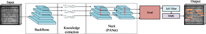
Flow chart of PV cell defect detection.
The process of detecting photovoltaic cell electroluminescence (EL) images using a deep learning model is depicted in Fig. 1. Initially, the EL images are input into a neural network for feature extraction, generating hierarchical features at varying resolutions. Subsequently, regional and semantic association information is derived from these multi-level features. A feature pyramid is then employed to fuse and enhance the representational capabilities of the features. In the final stage, these enhanced features are passed through the detection head to produce the prediction results. The discrepancy between the predicted outcomes and the ground truth is backpropagated through the network, facilitating the update of model parameters.
Our model employs YOLO13 as the baseline architecture, chosen for its robust performance and strong generalization capabilities, which have contributed to its widespread adoption in industrial applications14. However, YOLO is limited in its ability to model global context and capture regional and semantic relationships15. To overcome this limitation, we enhanced the backbone and neck components of YOLO, resulting in a photovoltaic cell defect detection model capable of topological knowledge extraction.
The detailed architecture of the model is illustrated in Fig. 2. In this diagram, the CBS module represents the sequence of Convolution, Batch Normalization, and Activation functions. The C2F module corresponds to the standard feature extraction module from YOLO V816. The Detect Head refers to a standard decoupled detection head. The operations of feature map concatenation and upsampling are denoted by Concat and Upsample, respectively.

Diagram of the model’s specific structure.
A multi-scale dynamic context-based feature extraction method for photovoltaic cell defects(backbone)

The structure of the backbone network.
Feature extraction from defective photovoltaic cell images typically follows a hierarchical structure. In the initial, shallow layers of the backbone network, the model captures fundamental features such as edges and color gradients. As the network deepens, the extracted features become increasingly complex, encompassing textures, shapes, and other intricate patterns, which are eventually abstracted into higher-level features essential for object recognition. Consequently, the backbone network is organized into four distinct stages, each dedicated to extracting features at varying levels of abstraction, thereby optimizing the efficiency and effectiveness of the feature extraction process. The backbone network itself is architected by sequentially stacking modules designed around multi-scale dynamic context feature extraction (MSCA), as depicted in Fig. 3.
Building upon the inspiration drawn from the CoT Transformer17, we introduce a novel feature extraction module, termed Multi-Scale Contextual Attention (MSCA), which is embedded at each stage of the neural network to enhance the extraction of defect features.
Traditional convolutional neural networks (CNNs) primarily capture target features by focusing on local region perception, which leads to uniform extraction of global information across regions containing the target. This approach, however, constrains the model’s ability to selectively extract features specific to the target18. In contrast, transformers employ a global attention mechanism, specifically utilizing a multi-head attention architecture to identify and learn from the most informative local regions. Despite this advantage, transformers inherently lack the convolutional inductive bias and local perception inherent to CNNs, resulting in a diminished capacity for spatial locality. Furthermore, the reliance on fully connected attention mechanisms imposes substantial computational overhead, particularly when processing high-resolution images. Moreover, both CNNs and transformers often fail to incorporate the rich dynamic context information present in the vicinity of key regions, which is critical for enhancing feature representation.
To address these challenges, we propose a feature extraction model that effectively captures dynamic multi-stage contextual information by leveraging the synergistic strengths of convolutional and attention mechanisms. This approach enables our model to precisely extract photovoltaic cell defect features, even within complex background environments, by dynamically integrating multi-stage contextual cues (Fig. 4).

Structure of the Dynamic Multi-Stage Context Feature Extraction Module.
Initially, convolutional filters are employed to encode local contextual information, resulting in the extraction of static contextual features. These features serve as the foundation for deriving the query (q), key (k), and value (v) components within the attention mechanism, as formulated below:
The value and key are derived using convolutional kernels with size of 1 and 3, respectively. ({text{BN}}( cdot ))and({text{ReLU}}( cdot ))are respectively batch normalization and activation functions; ({text{Con}}{{text{v}}_{k times k}}( cdot )) represents the convolution operation and k represents the convolution kernel size.
Then, concatenate the input(x in {{text{R}}^{b,c,h,w}})and static context(k in {{text{R}}^{b,c,h,w}})to obtain the output:
where(oplus)represents two tensors spliced along the channel dimension. To address the issue of the model excessively focusing on isolated local regions, we introduced a novel multi-head attention mechanism. Traditional attention mechanisms typically achieve multi-head attention by employing multiple independent sets of parallel linear projections. In contrast, our approach leverages a convolutional architecture, enabling the design of a multi-head attention mechanism that facilitates localized sparse perception within small regions. This design allows for the aggregation of richer multi-scale contextual information. The aforementioned computations are implemented through a multi-scale perception module, the detailed structure of which is illustrated in Fig. 5.

Detailed structure.
The design of the multi-scale perception block follows a streamlined approach. Initially, a bottleneck layer utilizing 1 × 1 convolution is employed to reduce the dimensionality of the input channels. This layer is strategically guided by the input features to encode static context and generate dynamic context. Subsequently, the output is processed by the multi-scale perception module, which employs convolutional kernels of varying sizes and dilation rates to extract multi-scale contextual information through multi-head attention mechanisms. This design aims to enhance the capture of local structures and texture information across diverse receptive fields, as illustrated by the following representation:
Here, (f( cdot ))represents convolution, k denotes the convolution kernel size, and Dia represents the dilation rate, (tilde {k}) represents the result after capturing the multi-scale context for (hat {k}).
Next, utilizing a convolutional layer, the multiple head features are compressed, and aggregation of features from (tilde {k})independent heads is achieved through spatial dimension averaging and normalization operations, resulting in the dynamic context matrix, specifically represented as:
where, ({text{Sigmoid}}( cdot ))represents for Sigmoid activation function; ({text{Mean}}( cdot ))represents for the operation of finding the mean.
Then, the results after self-attention are obtained by tensor multiplication blending. Ultimately, ({k_d}) is the output that aggregates the multi-scale dynamic context information.
Here, (otimes)represents for matrix pairwise multiplication. Finally, by using SKnet to aggregate static keys with dynamic keys, the final result is obtained.

Structure of SKNet(The main purpose of this figure is to illustrate how dynamic and static keys are input into SKNet, hence the detailed structure of SKNet is omitted).
As illustrated in Fig. 6, the SKNet framework integrates dynamic and static keys by adaptively merging their respective features through the application of selective convolutional kernels, as comprehensively discussed in reference19.
Centered feature pyramid structure with spatial semantic enhancement(Neck)
To achieve more effective integration of multi-scale features and to enhance the model’s capability in detecting small objects, we developed the Centered Feature Pyramid with Spatial Semantic Enhancement (SSA-CFPN). This architecture is designed to merge multi-scale features extracted by the backbone network. As illustrated in Fig. 7, the SSA-CFPN builds upon the PANet architecture by taking inputs from four stages of the backbone network, subsequently applying spatial semantic enhancement to refine these features before they are passed to the detection heads.
Initially, features extracted from the first three stages of the network are fed into the Semantic Relation Enhancement Module, while the features from the final stage are processed by the Explicit Visual Center (EVC) module. The Semantic Relation Enhancement Module is inspired by the principles of knowledge graphs and leverages graph neural networks to refine the semantic relationships between regions. It utilizes sparse region attention mechanisms to effectively capture multi-level semantic information across different resolution feature maps.
For the higher-resolution features obtained from the first three stages, we compute region and semantic correlations, integrating high- and low-resolution semantic correlation information through SKNet, in accordance with the fusion methodology outlined in the preceding section. The EVC module20 plays a critical role in aggregating global contextual information, thereby capturing long-range dependencies. Additionally, it enhances the aggregation of corner information to mitigate the risk of missing essential features. By fusing global and corner information, the EVC module generates and outputs higher-order representations of the image data, thereby contributing to more accurate and comprehensive feature extraction.

Structure of SSA-CFPN.
Explicit visual center module (EVC)
The structure of the Explicit Visual Center (EVC) module, as illustrated in Fig. 8, consists of two parallel cascaded sub-modules: the Global Information Aggregation module and the Corner Information Aggregation module. The Global Information Aggregation module is designed to capture coarse-grained spatial dependencies, or global information, across the entire image. Conversely, the Corner Information Aggregation module is specialized in enhancing corner features that are often overlooked, which are critical for representing fine-grained local key information. In the context of defect detection in photovoltaic cell images, the preservation of local information is crucial, as the loss of such details can lead to the model failing to detect small-scale or blurred defects.

Structure of EVC.
To address the noise present in electroluminescence images, the features fed into these parallel cascaded modules undergo an initial smoothing process. This step is essential for noise elimination, feature quality enhancement, and reduction of interference. The smoothing layer utilizes a large convolutional kernel with a size of 7 × 7. Such large kernels are particularly effective in capturing features over a broader area, aggregating contextual information, and mitigating noise. Following this, the features are subjected to further refinement through batch normalization and activation function layers, which serve to enhance their representational capacity, as detailed below:
Subsequently, the processed features are fed into parallel modules for Global Information Aggregation and Corner Information Aggregation, enabling comprehensive computational analysis.
Global information aggregation module
The global information aggregation module is composed of parallel depth-wise separable convolutions21 and a C-MLP. Feature grouping and normalization are achieved through Group Normalization (GN), which significantly mitigates inter-feature interference. The operations within this module can be formally described as follows:
Where ({text{DWConv}}( cdot )) is the depth-separable convolution and ({text{GN}}( cdot )) is the group normalization. As illustrated in Fig. 9, the C-MLP module is composed of two linear layers, optimized for capturing cross-channel information, thereby enhancing its applicability in photovoltaic cell defect detection. This module integrates Cycle MLP22 layers and Channel MLP layers in a serial configuration to effectively capture both inter-channel interactions and spatial relationships, thereby improving the model’s ability to detect and characterize defects within photovoltaic cells.

Structure of C-MLP.
In this context, Cycle MLP integrates the concept of receptive fields with the multilayer perceptron (MLP) architecture. Specifically, it introduces spatial shifts S across the H×W dimensions, augmenting the traditional Channel MLP. The spatial shift S is adjustable, allowing for flexibility, and its computation parallels that of deformable convolutions. The shifting mechanism utilizes bilinear interpolation for precise feature alignment.
The aforementioned operations can be formally represented as follows:
Where ({text{ChannelMLP}}( cdot )) and ({text{CycleMLP}}( cdot )) are computational functions for Channel MLP and Cycle MLP, respectively.
Edge and corner information aggregation module
The features enhanced by the multi-layer local perception module may still overlook certain local regions, particularly given the subtle nature of defects in photovoltaic cells. To address this limitation and to more effectively extract comprehensive and high-level target features, we employ the Multi-layer Information Aggregation (MIA) module. This module aggregates local information within the feature maps, thereby augmenting the global information output by the multi-layer local perception module. The detailed architecture of the MIA module is depicted in Fig. 10. The input to the MIA consists of deep feature maps obtained from the final stage of the backbone network, which have been pre-processed through feature smoothing.

Structure of Edge and Corner Information Aggregation Module.
The features are initially subjected to a convolutional layer, which functions as a preliminary encoding preprocessing step. Following this, the processed features are input into the encoding module for further transformation and representation.The encoding module initially establishes a learnable parameter matrix({W_{code}}=[{b_1},{b_2}….{b_k}] in {R^{k,c}}), and a set of adjustable visual center scale factors ({W_s}=[{s_1},{s_2},….,{s_k}] in {R^k}), which correspond to ({W_{code}}). To enable the parameter matrix ({W_{code}}) to learn the edge and corner, or local positional information in ({X_c}), the information of the k-th group of the entire feature set can be represented as follows:
Specifically, ({x_i}) represents the i-th pixel, and ({b_k}) is the k-th learnable encoding parameter. By computing the difference between the two, the positional information of each pixel relative to the learnable encoding can be extracted. The L2 norm is employed as a regularization technique to impose constraints on model parameters, thereby mitigating the risk of overfitting. k is the total number of visual centers, similar to the multiple heads in a multi-head attention mechanism. This multi-group encoding strategy facilitates the comprehensive capture of local information by employing multiple encoding pathways, thereby mitigating the risk of excessive attention aggregation and ensuring a more balanced and nuanced feature representation. Then, the BRM (Batch Normalization, ReLU, and Mean) is used to fuse all ({e_k}), where ({text{BRM}}( cdot )) includes a BN layer, ReLU layer, and averaging operation, represented as follows:
Upon obtaining the output e, it is subsequently passed through a fully connected layer followed by a convolutional layer with a kernel size of 1, aiming to predict features associated with locally sensitive information. This process can be formally represented as:
Where({text{f}}{{text{c}}_1}())represents the fully connected layer, and ({text{Con}}{{text{v}}_{1 times 1}}()) is used to adjust the number of channels. In essence, the described operations are designed to learn the significance of individual pixels in order to capture long-range dependencies across channels. Features with diminished local information are assigned lower weights, while those that exhibit greater sensitivity to local information are emphasized, thereby enhancing the representation of local details. Subsequently, following the application of these weights to each channel of the feature map, a channel-wise element-wise addition is performed between the global and local features, resulting in the final output of the Edge and Corner Visualization (ECV) module.
Semantic relationship enhancement module based on graph neural networks(SRE)
To address the limitations of conventional convolutional and attention-based object detection models, which capture global spatial dependencies but often neglect correlations between different semantic regions, we propose a Semantic Relationship Enhancement Module grounded in Graph Neural Networks (GNNs). This module is designed to extract semantic spatial knowledge from EL (Electroluminescence) images, facilitating a deeper understanding and more accurate classification of various features within these images. For example, the module is capable of distinguishing between micro-cracks, broken fingers, and gray spots across different defect types. By enhancing semantic understanding, the module significantly improves the accuracy and reliability of defect classification.
The Semantic Relationship Enhancement Module operates through three key steps: first, it constructs a topological graph that represents relationships between different regions of the image; second, it performs sparse self-attention calculations based on this graph; and finally, it aggregates semantic information from each region. Subsequently, graph convolutional operations are applied according to the constructed topological graph, enabling the extraction and enhancement of semantic relationships between the regions, thereby improving the model’s overall performance in defect detection and classification.
Construction of spatial topological graph
As illustrated in Fig. 11, the image is initially partitioned into s×s windows. For each region, the k most associated regions are identified to construct an adjacency matrix, which explicitly represents the interrelationships between the target regions. Leveraging these relationships, semantic association computations are then conducted between the local regions, enabling a more refined understanding of the spatial dependencies within the image.

Finding Routing Between Regions.

The calculation process of inter-region indexing relationships.
The process of computing routing between regions is depicted in Fig. 12, where, for simplicity, only a single-input single-head self-attention mechanism is employed.
Given a feature map (x in {R^{C times H times W}}), first divide it into S×S sub-regions, where each sub-region’s feature block has (HW/{S^2}) pixels, with each pixel representing a feature vector. Reformat the input as ({x_i} in {R^{{s^2} times HW/{S^2} times C}}). Next, construct a directed graph to find the region that each given region should correspond to with the highest degree of association. Begin by obtaining queries, keys, and values in attention through convolution, representing fine-grained analysis of regions and aggregating region-level contextual information:
Then compute the average of queries Q and keys K for each region, resulting in ({Q_i},{K_i} in {R^{{s^2} times C}}), represented as:
Represents the aggregation of semantic information within each region. Then, derive the adjacency matrix to capture the region-level relationships between Q and K:
The adjacency matrix({A_i} in {R^{{s^2} times {s^2}}})represents the semantic correlation between two regions, where ({A_i}) denotes the association of each region with all other regions. Therefore, it is necessary to retain only the top-k regions with the highest relevance for each region to obtain the routing index matrix, denoted as:
Where ({text{Top}} – k( cdot )) is the function used to select the most relevant k regions. In matrix ({I_i} in {R^{{s^2} times k}}), the i-th row of the routing index matrix represents the top k regions that are most highly associated with the i-th region.
Spatial enhanced attention computation
In the previous section, we obtained the spatial relationships between regions. Next, as illustrated in Fig. 13, we calculate spatial attention selectively among highly correlated regions to enhance spatial information24. Initially, using function(gather()), we locate the required keys and values based on these relationships:

Spatial sparse attention computation.
Then, attention calculation proceeds as follows:
where ({text{Softmax}}( cdot )) is the function used to select the most relevant k regions.
Semantic topological enhancement computation
In the preceding section, we focused on spatially-enhanced attention computation. However, this approach primarily augments the spatial dimensions of the information while overlooking the effective extraction of long-range topological correlations. To address this limitation, we integrate a knowledge graph into the object detection framework, enabling the extraction of semantic relationships between indexed regions and leveraging these relationships for region-specific feature enhancement.
As depicted in Fig. 14, the adjacency matrix and node vectors are input into a Graph Convolutional Network (GCN) to extract contextual relational information embedded within the graph structure. The node vectors are derived by averaging the features across the channel dimension for each window, thereby facilitating the GCN in capturing and enhancing the semantic relationships within the image.

Topological information enhancement computation.
The specific formula for constructing node vectors is as follows:
Then, we compute the degree matrix D of the adjacency matrix A. The degree matrix D represents the sum of edges connected to each node in the graph:
The adjacency matrix A is represented as:
Then, decompose the Laplacian matrix of the graph, where the role of the degree matrix D is to prevent the problem of gradient vanishing or exploding, effectively normalizing the Laplacian matrix, expressed as:
Therefore, the computation of graph convolution can be represented as:
Therefore, where ({W_g}) denotes learnable weight parameters. Ultimately, the output shape of the graph convolution operation remains consistent with its input, with each window corresponding to a vector of channel length. This ensures that the output effectively captures the weights associated with each window across all channels, thereby facilitating the interaction between knowledge relationships and cross-channel information. To further refine this process, we apply an additional layer of weighting, informed by the results of spatial attention computation, culminating in the final output. This approach enhances the integration of semantic relationships with spatial and channel-wise information, leading to improved feature representation and detection accuracy.
Experiments
In this section, we conduct detailed ablation and comparative experiments on the model improvements using a publicly available electroluminescence dataset. Additionally, we visually illustrate the impact of the improvements on model performance.
Photovoltaic cell electroluminescence image dataset
As illustrated in Fig. 15, we utilized the publicly available PVEL-AD25 photovoltaic cell electroluminescence (EL) imaging dataset as the foundational dataset for our research. This dataset comprises a diverse set of near-infrared images, capturing various internal defects and inhomogeneous backgrounds, totaling 3,751 images across eleven distinct types of anomalous defects. These defects include cracks, finger breaks, black kernels, horizontal and vertical mismatches, thick lines, scratches, fragments, fragmented corners, and short-circuit defects.

Part of the EL imaging PV cell defect dataset.
Given the rarity of certain defect categories within the dataset, their inclusion would result in a highly imbalanced and impractical dataset distribution. To address this issue, we excluded some of the less prevalent defect categories, retaining only five common defect types: broken fingers, cracks, thick lines, horizontal misalignments, and black cores.
Recognizing that the performance of deep learning models is closely tied to the quantity and quality of the training data, and considering the category imbalance and insufficient data volume in the original dataset, we applied various data augmentation techniques. These techniques included radial transform, Gaussian blur, mosaic data augmentation, and color dithering. The distribution of the augmented dataset is presented in Fig. 16, resulting in a total of 13,084 EL images of defective photovoltaic cells.

Enhanced PV cell data distribution(The numbers in the table represent the number of labels for each category of defects, A and B represent before and after data enhancement, respectively.)
Evaluation indicators
In this paper, two commonly used indicators are used to evaluate the performance of the model, namely precision P and recall R. Higher evaluations indicate higher performance, and vice versa.
There are four types of target detection models: true positive (TP), true negative (TN), false positive (FP), and false negative (FN). The accuracy rate is used to evaluate the accuracy of the detection model. The recall rate is used to evaluate the ability of the test model to identify all positive samples. The mAP is the average accuracy of all categories. The higher mAP value, the better the comprehensive performance of the model, where n is the number of categories. The average precision (AP) is used to evaluate the precision rate of a certain type of target detection model, where p is the precision rate and r is the recall rate.
Implementation details
To fully exploit the performance of the model, we first pre-train the model on the COCO2017 dataset and produced a pre-trained model.
Subsequently, 80% of the PV cell defects dataset was selected as the training set, 20% as the validation set, and stratified sampling was used to randomly divide the original data, while retaining the sample distributions of the samples within the different categories in the training and test sets, and load the pre-training model, where the hyper-parameters were set as in Table 1.
The experiments run on a Windows 10 computer with an AMD 5600X CPU, two RTX8000 GPUs, and 32G of RAM, using the Pycharm platform.
Experimental results
In this section, we present the main experimental results in three parts. Firstly, we compare the state-of-the-art methods to verify the advantages of our model. Secondly, we conduct an ablation study to investigate the role of the module. Finally, we perform visualization experiments on each module to visually demonstrate the effects brought by the module.
Comparison with other detection methods
To evaluate the performance advantages of our model, we conducted a comparative analysis against nine mainstream object detection models: Deformable DETR, YOLOv5, YOLOv7, YOLOv8, YOLO-X, PicoDet, Cascade-RCNN, Faster-RCNN, and Sparse-RCNN. Each model was trained on the same dataset and assessed on the identical test set under consistent conditions. As presented in Table 2, all detection models demonstrated varying levels of missed detections under these conditions. Notably, our model exhibited the fewest missed detection targets, indicating superior detection performance. The data further suggests that our model’s evaluation metrics surpass those of several other detection models, highlighting its enhanced performance. In the context of industrial defect detection, recall rate metrics are of paramount importance. Our model demonstrates a significant advantage in recall rate compared to other models, resulting in lower missed detection rates and proving its efficacy in practical applications.
Under identical conditions, each detection model demonstrates varying levels of missed detections. Our model, however, exhibits fewer missed targets and achieves relatively higher detection accuracy, underscoring its superior performance. This improvement can be attributed to the distinct feature extraction networks and fusion methods employed by different detection models, which result in varied learning and representation of defect information. Furthermore, the input image sizes used during model training differ across models, which also influences performance outcomes. In our study, we optimized the detection examples and the model training environment, ensuring an ideal configuration. Therefore, the metrics provided should be considered for reference purposes only, as they reflect the specific conditions under which the models were evaluated.
The loss curve during the training process
The training process of the model is depicted by the loss curve in Fig. 17. Overall, the loss of our model demonstrates a clear decreasing trend, eventually stabilizing in the later stages. Both the validation and training losses converge, indicating that the model reaches a stable and convergent state.
In the initial 50 epochs, the loss decreases rapidly, accompanied by a swift improvement in accuracy. After 50 epochs, although the rate of loss reduction slows down, it remains significant. Beyond this point, the loss reduction becomes more gradual, with slight fluctuations within a certain range, but the overall downward trend persists. This pattern continues until approximately the 220th epoch, where the loss stabilizes. By the 250th epoch, the loss curve flattens out, indicating that the loss has reached its minimum, and the model has effectively converged, exhibiting optimal performance.
he accuracy curve mirrors the general trend of the loss curve, though with larger fluctuations during the first 75 epochs. In these early epochs, accuracy improves significantly; however, recall and mean average precision (mAP) remain relatively low. This can be attributed to the model’s rapid convergence when identifying simpler defects, such as black cores, which leads to an early bias in predictions towards this defect category. The detection of more complex defect types poses greater challenges, resulting in imbalanced detection performance across different categories during the initial training stages.
Between the 80th and 120th epochs, the model’s accuracy and recall increase steadily, with the rate of improvement gradually slowing and fluctuations diminishing, indicating increased model stability. After 150 epochs, significant improvements in accuracy and recall plateau, and the metrics remain somewhat unstable. It is not until after 270 epochs of training that the model’s accuracy and recall stabilize fully, with the curves flattening out, signifying that the model has converged and achieved consistent performance by this stage.

The curve of the loss and the change of each evaluation index during the experiment (Top-left: The loss curves for the training set, with red, blue, and green representing the bounding box loss, confidence loss, and classification loss, respectively. Bottom-left: The loss curve for the validation set. Top-right: The curves showing the changes in precision and recall. Bottom-right: The curve showing the changes in mean average precision (mAP)).
As depicted in Fig. 18, we validated the model’s performance on the test set and visualized the detection results across various defect categories. Figure 19 presents the detection accuracy for each defect type. Due to the distinct and straightforward characteristics of black cores and horizontal misalignments, our model achieved Average Precisions (APs) of 99.0% and 99.5% for these defect types, respectively. Notably, the model demonstrated exceptional performance with virtually no false detections or missed detections for these categories, underscoring its robustness in identifying these specific defects.

Experimental result (The results of the model detecting various defects, including a total of five defect types, demonstrate that the model essentially has no missed detections or false detections.)

AP of defect detection for each category(The model’s detection accuracy for several defect types shows that the accuracy for black core and horizontal misalignment is relatively high, at 99% and 99.5%, respectively, while the accuracy for cracks is comparatively lower, at 77.2%.)
For small targets such as broken fingers, cracks, and thick lines, the model achieved mean Average Precisions of 90.7%, 77.2%, and 90.7%, respectively. These results indicate that the model was effective in detecting the majority of defect targets while maintaining relatively high precision. The improvements we proposed have significantly enhanced the model’s capability to detect small-scale and less conspicuous defects, thereby meeting the stringent requirements of industrial applications. The relatively lower accuracy observed for cracks can be attributed to their subtle characteristics, which make them more susceptible to interference from background noise and false positives.
Ablation experiments
This section evaluates the effectiveness of each proposed improvement by conducting ablation experiments to assess the contributions of different modifications to the model’s overall performance. All experiments were conducted using the YOLOv5 model as the baseline. Initially, the C3 module in the YOLOv5 backbone network was replaced with the dynamic multi-scale context-aware feature extraction module (MSCA). As indicated in Table 3, the introduction of the MSCA resulted in an increase in precision and recall by 0.6% and 0.4%, respectively, demonstrating enhanced feature extraction capabilities. The convolution-based attention mechanism in MSCA effectively aggregates the texture structures of local defects and differentiates between pixel points, making it particularly adept at detecting less conspicuous photovoltaic cell defects. This improvement underscores the suitability of the MSCA module for applications requiring precise detection of subtle defects.
The visualization of the MSCA module
As shown in Fig. 20, detecting small-scale defects poses a significant challenge in photovoltaic cell defect detection. Due to the low contrast in electroluminescence images, conventional convolutional neural networks tend to miss these features, resulting in missed or false detections. Our feature extraction method effectively captures the relationships between local keys and queries, enriching the extraction of multi-level contextual information around each pixel. This enhances the extraction of texture boundary information, thereby effectively preventing information loss and improving the detection performance for small targets. We also visualize the feature map as a 3D histogram, which can more intuitively represent the effect of the proposed method on the extraction of key features, and the higher z-axis region in the 3D histogram represents the features that the model focuses on. As can be seen from these 3D histograms, our method is effective in suppressing background features and highlighting critical defective regions.

Feature map (The left subfigure represents the experimental results output by the model, while the right subfigures display different feature maps. These include the feature maps from the baseline model and our proposed method. Each subfigure illustrates the feature activation in specific regions, with the green highlighted areas indicating where the model has detected certain critical features, potentially associated with defects.)
The visualization of the SRE module
For less prominent defects such as cracks, as shown in Fig. 21, the improved backbone network can better aggregate features of these small and less textured defects. Compared to other types of defects, detecting cracks presents the greatest challenge. The EVC module is capable of modeling a larger receptive field and capturing global dependencies, enabling the model to learn points of interest. As a result, it achieves significant performance improvements.

Feature map and result(The figure illustrates the changes in model detection results and feature maps before and after adding the ECV module. It is evident that the ECV module enhances the model’s ability to detect low-contrast defects such as cracks, with the extracted features becoming more precise and prominent.)
The visualization of the MSCA module
As shown in Fig. 22, we visualized the routing relationships between regions, where each region establishes routing indices with the top k other regions. From the figure, it can be observed that the constructed graph structure changes during the training process. This indicates that the model can adaptively model the semantic associations between regions at different feature resolutions based on the circumstances.

The topological graph of associations between local regions(The 3D topological maps in the figure are generated from the electroluminescence image on the left, where S = 4, resulting in a total of 16 windows. The information within each window is aggregated to represent 16 nodes. The two topological maps on the right represent two different types of region-level spatial semantic association information.)
As shown in Fig. 23, we visualize the regional semantic information before and after applying graph neural networks (for clearer visualization, larger-scale targets are selected). Clearly, the graph neural network captures correlations between regions, enhancing the differentiation between background and targets. There is a significant difference in the distinguishability between regions with dark nuclei (black) and regions without targets (white) before and after graph convolution.

Visualizing semantic information of local regions(In the figure, the second and third 3D images from left to right represent the averaged region information, respectively, and each node is the mean value of the region information, where S = 4, resulting in a total of 16 windows.)
As shown in Fig. 24, we visualize the results using a greater number of local windows (s = 7). A higher number of local windows enhances the detection of fine targets such as cracks or fractures. The regions outlined in red boxes in the figure indicate areas with defective targets. The semantic information from the two three-dimensional visualizations shows results after different layers of graph convolution. Through observation, our method effectively captures the semantic relationships in this region, enhancing the differentiation between areas with and without targets in the background, thus achieving good detection performance.

Visualizing semantic information of local regions(The results for more windows are visualized in the figure, where S = 7 and contains a total of 49 windows, with the red boxes representing the windows corresponding to the regions with defects.)
The changes in semantic-enhanced feature maps are depicted in Fig. 25, demonstrating the significant effectiveness of our method in feature enhancement, resulting in performance improvements of 0.8% and 0.6%.

Visualizing feature map(The figure illustrates the change in the feature map after the SRE module.)
Conclusion
We propose a photovoltaic cell defect detection model capable of extracting topological knowledge, aggregating local multi-order dynamic contexts, and effectively capturing diverse defect features, particularly for small flaws. Additionally, by integrating a visual center module that merges global and local information, the model focuses on coarse-grained semantic information while preserving fine-grained features in corners. Finally, through constructing spatial semantic topological maps of defect images, sparse spatial attention computations are implemented, and semantic knowledge between regions is extracted using graph convolution, achieving precise defect detection.
However, despite achieving certain performance advantages, our model exhibits lower training efficiency. Therefore, further optimization potential exists in lightweighting when considering mobile and embedded devices.
Data availability
Publicly available data supporting the conclusions of this study can be found at: https://github.com/binyisu/PVEL-AD.
References
-
Zhao, S., Chen, H., Wang, C., Zhou, Y. & Zhang, Z. S. S. N. Shift suppression network for endogenous shift of photovoltaic defect detection. IEEE Trans. Ind. Inf. 20, 4685–4697 (2024).
Google Scholar
-
Tsai, D. M., Wu, S. C. & Chiu, W. Y. Defect detection in solar modules using ICA basis images. IEEE Trans. Ind. Inf. 9, 122–131 (2013).
Google Scholar
-
Dhimish, M., d’Alessandro, V. & Daliento, S. Investigating the impact of cracks on solar cells performance: analysis based on nonuniform and uniform crack distributions. IEEE Trans. Ind. Inf. 18, 1684–1693 (2021).
Google Scholar
-
Zhang, J. et al. Automatic detection of defective solar cells in electroluminescence images via global similarity and concatenated saliency guided network. IEEE Trans. Ind. Inf. 19, 7335–7345 (2022).
Google Scholar
-
Dhimish, M. et al. The impact of cracks on photovoltaic power performance. J. Sci. Adv. Mater. Devices. 2, 199–209 (2017).
Google Scholar
-
Tomanek, P., Skarvada, P., MacKu, R. & Grmela, L. Detection and localization of defects in monocrystalline silicon solar cell. Adv. Opt. Technol. (2010). (2010).
-
Tsai, D. M. & Molina, D. E. R. morphology-based defect detection in machined surfaces with circular tool-mark patterns. Measurement. 134, 209–217 (2019).
Google Scholar
-
Zhang, J. et al. Fast object detection of anomaly photovoltaic (PV) cells using deep neural networks. Appl. Energy. 372, 123759 (2024).
Google Scholar
-
Xu, Q. et al. Adaptive working condition recognition with clustering-based contrastive learning for unsupervised anomaly detection. IEEE Trans. Ind. Inf. (2024).
-
Liu, Y. et al. Deep learning-based method for defect detection in electroluminescent images of polycrystalline silicon solar cells. Opt. Express. 32, 17295–17317 (2024).
Google Scholar
-
Zhu, J. et al. C2DEM-YOLO: improved YOLOv8 for defect detection of photovoltaic cell modules in electroluminescence images. Nondestruct Test. Eval 1–23 (2024).
-
Liu, Q. et al. A real-time anchor-free defect detector with global and local feature enhancement for surface defect detection. Expert Syst. Appl. 246, 123199 (2024).
Google Scholar
-
Redmon, J., Divvala, S., Girshick, R. & Farhadi, A. You only look once: Unified, real-time object detection. In Proceedings of the IEEE Conference on Computer Vision and Pattern Recognition 779–788 (2016).
-
Hussain, M. YOLO-v1 to YOLO-v8, the rise of YOLO and its complementary nature toward digital manufacturing and industrial defect detection. Machines. 11, 677 (2023).
Google Scholar
-
Zhang, Z. et al. ViT-YOLO: Transformer-based YOLO for object detection. In Proceedings of the IEEE/CVF International Conference on Computer Vision 2799–2808 (2021).
-
Varghese, R. & Sambath, M. YOLOv8: A novel object detection algorithm with enhanced performance and robustness. In 2024 International Conference on Advances in Data Engineering and Intelligent Computing Systems (ADICS) 1–6IEEE, (2024).
-
Li, Y. et al. Contextual transformer networks for visual recognition. IEEE Trans. Pattern Anal. Mach. Intell. 45, 1489–1500 (2022).
Google Scholar
-
Han, K. et al. Transformer in transformer. Adv. Neural Inf. Process. Syst. 34, 15908–15919 (2021).
-
Wu, W. et al. SK-Net: Deep learning on point cloud via end-to-end discovery of spatial keypoints. In Proceedings of the AAAI Conference on Artificial Intelligence 34, 6422–6429 (2020).
-
Quan, Y. et al. Centralized feature pyramid for object detection. IEEE Trans. Image Process. (2023).
-
Chollet, F. & Xception Deep learning with depthwise separable convolutions. In Proceedings of the IEEE Conference on Computer Vision and Pattern Recognition 1251–1258 (2017).
-
Chen, S. et al. CycleMLP: a MLP-like architecture for dense prediction. arXiv Preprint arXiv :210710224 (2021).
-
Kipf, T. N. & Welling, M. Semi-supervised classification with graph convolutional networks. arXiv Preprint arXiv :160902907 (2016).
-
Zhu, L. et al. Biformer: Vision transformer with bi-level routing attention. In Proceedings of the IEEE/CVF Conference on Computer Vision and Pattern Recognition 10323–10333 (2023).
-
Su, B., Zhou, Z. & Chen, H. PVEL-AD: a large-scale open-world dataset for photovoltaic cell anomaly detection. IEEE Trans. Ind. Inf. 19, 404–413 (2022).
Google Scholar
-
Wu, Y. et al. Rethinking classification and localization for object detection. arXiv preprint arXiv:1904.06493 (2019).
-
Ge, Z. et al. YOLOX: Exceeding YOLO series in 2021. arXiv Preprint arXiv: 210708430 (2021).
-
Sun, P. et al. Sparse R-CNN: End-to-end object detection with learnable proposals. arXiv preprint arXiv:2011.12450 (2020).
-
Wang, C. Y., Bochkovskiy, A. & Liao, H. Y. M. YOLOv7: trainable bag-of-freebies sets new state-of-the-art for real-time object detectors. arXiv Preprint arXiv :220702696 (2022).
-
Zhu, X. et al. Deformable DETR: Deformable transformers for end-to-end object detection. arXiv preprint arXiv:2010.04159 (2020).
-
Redmon, J. You only look once: Unified, real-time object detection. In Proceedings of the IEEE Conference on Computer Vision and Pattern Recognition (2016).
-
Liu, W. et al. Springer International Publishing,. SSD: Single shot multibox detector. In Computer Vision–ECCV 2016: 14th European Conference, Amsterdam, The Netherlands, October 11–14, 2016, Proceedings, Part I 14 21–37 (2016).
-
Ren, S., He, K., Girshick, R., Sun, J. & Faster, R-C-N-N. Towards real-time object detection with region proposal networks. IEEE Trans. Pattern Anal. Mach. Intell. 39, 1137–1149 (2016).
Google Scholar
-
He, K., Gkioxari, G., Dollár, P. & Girshick, R. Mask R-CNN. In Proceedings of the IEEE International Conference on Computer Vision 2961–2969 (2017).
-
Scarselli, F., Gori, M., Tsoi, A. C., Hagenbuchner, M. & Monfardini, G. The graph neural network model. IEEE Trans. Neural Netw. 20, 61–80 (2008).
Google Scholar
-
Defferrard, M., Bresson, X. & Vandergheynst, P. Convolutional neural networks on graphs with fast localized spectral filtering. Adv. Neural Inf. Process. Syst. 29, (2016).
-
Velickovic, P. et al. Graph attention networks. Statistics 1050, 10–48550 (2017).
-
Liu, Q., Liu, M., Wang, C. & Wu, Q. M. J. An efficient CNN-based detector for photovoltaic module cells defect detection in electroluminescence images. Sol Energy. 267, 112245 (2024).
Google Scholar
-
Zhao, S., Chen, H., Wang, C., Zhou, Y. & Zhang, Z. RGR-Net: Refined graph reasoning network for multi-height hotspot defect detection in photovoltaic farms. Expert Syst. Appl. 245, 123034 (2024).
Google Scholar
-
Zhao, S., Chen, H., Wang, C. & Zhang, Z. S. S. N. Shift suppression network for endogenous shift of photovoltaic defect detection. IEEE Trans. Ind. Inf. 20, 4685–4697 (2024).
Google Scholar
Author information
Authors and Affiliations
Contributions
Contribution Statement: Conceptualization: Q, L, and Z conceived and designed the study.Methodology: L and Z conducted the experiments and data collection.Formal analysis: L performed the statistical analysis and interpreted the data.Writing – original draft preparation: L wrote the initial draft of the manuscript.Writing – review and editing: All authors reviewed and edited the manuscript critically for important intellectual content.Resources: Q,X, D,F provided experimental facilities and materials.
Ethics declarations
Competing interests
The authors declare no competing interests.
Additional information
Publisher’s note
Springer Nature remains neutral with regard to jurisdictional claims in published maps and institutional affiliations.
Rights and permissions
Open Access This article is licensed under a Creative Commons Attribution-NonCommercial-NoDerivatives 4.0 International License, which permits any non-commercial use, sharing, distribution and reproduction in any medium or format, as long as you give appropriate credit to the original author(s) and the source, provide a link to the Creative Commons licence, and indicate if you modified the licensed material. You do not have permission under this licence to share adapted material derived from this article or parts of it. The images or other third party material in this article are included in the article’s Creative Commons licence, unless indicated otherwise in a credit line to the material. If material is not included in the article’s Creative Commons licence and your intended use is not permitted by statutory regulation or exceeds the permitted use, you will need to obtain permission directly from the copyright holder. To view a copy of this licence, visit http://creativecommons.org/licenses/by-nc-nd/4.0/.
Reprints and permissions
About this article
Cite this article
Qu, Z., Li, L., Zang, J. et al. A photovoltaic cell defect detection model capable of topological knowledge extraction.
Sci Rep 14, 21904 (2024). https://doi.org/10.1038/s41598-024-72717-0
-
Received: 18 July 2024
-
Accepted: 10 September 2024
-
Published: 19 September 2024
-
DOI: https://doi.org/10.1038/s41598-024-72717-0
Keywords
- Defect detection
- Deep learning
- Transformer
- Photovoltaic cell
Comments
By submitting a comment you agree to abide by our Terms and Community Guidelines. If you find something abusive or that does not comply with our terms or guidelines please flag it as inappropriate.