Abstract
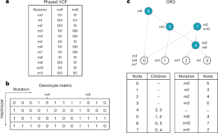
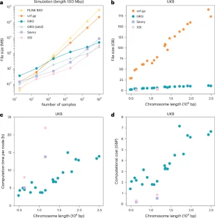
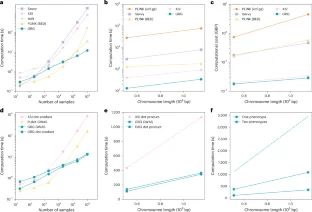
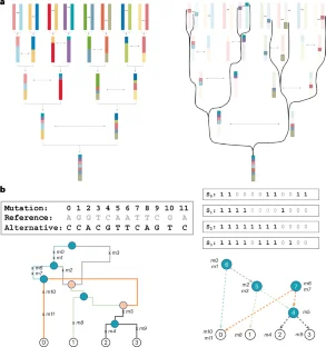
Computational analysis of a large number of genomes requires a data structure that can represent the dataset compactly while also enabling efficient operations on variants and samples. However, encoding genetic data in existing tabular data structures and file formats has become costly and unsustainable. Here we introduce the genotype representation graph (GRG), a fully connected hierarchical data structure that losslessly encodes phased whole-genome polymorphisms. Exploiting variant-sharing across samples enables GRG to compress 200,000 UK Biobank phased human genomes to 5–26 gigabytes per chromosome, also enabling graph-traversal algorithms to reuse computed values in random access memory. Constructing and processing GRG files scales to a million whole genomes. Using allele frequencies and association effects as examples, we show that computation on GRG via graph traversal runs the fastest among all tested alternatives. GRG-based algorithms have the potential to increase the scalability and reduce the cost of analyzing large genomic datasets.
This is a preview of subscription content, access via your institution
Access options
/* style specs end */
Access Nature and 54 other Nature Portfolio journals
Get Nature+, our best-value online-access subscription
$29.99 / 30 days
cancel any time
Subscribe to this journal
Receive 12 digital issues and online access to articles
$99.00 per year
only $8.25 per issue
Buy this article
- Purchase on SpringerLink
- Instant access to full article PDF
Prices may be subject to local taxes which are calculated during checkout
/* style specs start */
style {
display: none !important;
}
.LiveAreaSection * {
align-content: stretch;
align-items: stretch;
align-self: auto;
animation-delay: 0s;
animation-direction: normal;
animation-duration: 0s;
animation-fill-mode: none;
animation-iteration-count: 1;
animation-name: none;
animation-play-state: running;
animation-timing-function: ease;
azimuth: center;
backface-visibility: visible;
background-attachment: scroll;
background-blend-mode: normal;
background-clip: borderBox;
background-color: transparent;
background-image: none;
background-origin: paddingBox;
background-position: 0 0;
background-repeat: repeat;
background-size: auto auto;
block-size: auto;
border-block-end-color: currentcolor;
border-block-end-style: none;
border-block-end-width: medium;
border-block-start-color: currentcolor;
border-block-start-style: none;
border-block-start-width: medium;
border-bottom-color: currentcolor;
border-bottom-left-radius: 0;
border-bottom-right-radius: 0;
border-bottom-style: none;
border-bottom-width: medium;
border-collapse: separate;
border-image-outset: 0s;
border-image-repeat: stretch;
border-image-slice: 100%;
border-image-source: none;
border-image-width: 1;
border-inline-end-color: currentcolor;
border-inline-end-style: none;
border-inline-end-width: medium;
border-inline-start-color: currentcolor;
border-inline-start-style: none;
border-inline-start-width: medium;
border-left-color: currentcolor;
border-left-style: none;
border-left-width: medium;
border-right-color: currentcolor;
border-right-style: none;
border-right-width: medium;
border-spacing: 0;
border-top-color: currentcolor;
border-top-left-radius: 0;
border-top-right-radius: 0;
border-top-style: none;
border-top-width: medium;
bottom: auto;
box-decoration-break: slice;
box-shadow: none;
box-sizing: border-box;
break-after: auto;
break-before: auto;
break-inside: auto;
caption-side: top;
caret-color: auto;
clear: none;
clip: auto;
clip-path: none;
color: initial;
column-count: auto;
column-fill: balance;
column-gap: normal;
column-rule-color: currentcolor;
column-rule-style: none;
column-rule-width: medium;
column-span: none;
column-width: auto;
content: normal;
counter-increment: none;
counter-reset: none;
cursor: auto;
display: inline;
empty-cells: show;
filter: none;
flex-basis: auto;
flex-direction: row;
flex-grow: 0;
flex-shrink: 1;
flex-wrap: nowrap;
float: none;
font-family: initial;
font-feature-settings: normal;
font-kerning: auto;
font-language-override: normal;
font-size: medium;
font-size-adjust: none;
font-stretch: normal;
font-style: normal;
font-synthesis: weight style;
font-variant: normal;
font-variant-alternates: normal;
font-variant-caps: normal;
font-variant-east-asian: normal;
font-variant-ligatures: normal;
font-variant-numeric: normal;
font-variant-position: normal;
font-weight: 400;
grid-auto-columns: auto;
grid-auto-flow: row;
grid-auto-rows: auto;
grid-column-end: auto;
grid-column-gap: 0;
grid-column-start: auto;
grid-row-end: auto;
grid-row-gap: 0;
grid-row-start: auto;
grid-template-areas: none;
grid-template-columns: none;
grid-template-rows: none;
height: auto;
hyphens: manual;
image-orientation: 0deg;
image-rendering: auto;
image-resolution: 1dppx;
ime-mode: auto;
inline-size: auto;
isolation: auto;
justify-content: flexStart;
left: auto;
letter-spacing: normal;
line-break: auto;
line-height: normal;
list-style-image: none;
list-style-position: outside;
list-style-type: disc;
margin-block-end: 0;
margin-block-start: 0;
margin-bottom: 0;
margin-inline-end: 0;
margin-inline-start: 0;
margin-left: 0;
margin-right: 0;
margin-top: 0;
mask-clip: borderBox;
mask-composite: add;
mask-image: none;
mask-mode: matchSource;
mask-origin: borderBox;
mask-position: 0 0;
mask-repeat: repeat;
mask-size: auto;
mask-type: luminance;
max-height: none;
max-width: none;
min-block-size: 0;
min-height: 0;
min-inline-size: 0;
min-width: 0;
mix-blend-mode: normal;
object-fit: fill;
object-position: 50% 50%;
offset-block-end: auto;
offset-block-start: auto;
offset-inline-end: auto;
offset-inline-start: auto;
opacity: 1;
order: 0;
orphans: 2;
outline-color: initial;
outline-offset: 0;
outline-style: none;
outline-width: medium;
overflow: visible;
overflow-wrap: normal;
overflow-x: visible;
overflow-y: visible;
padding-block-end: 0;
padding-block-start: 0;
padding-bottom: 0;
padding-inline-end: 0;
padding-inline-start: 0;
padding-left: 0;
padding-right: 0;
padding-top: 0;
page-break-after: auto;
page-break-before: auto;
page-break-inside: auto;
perspective: none;
perspective-origin: 50% 50%;
pointer-events: auto;
position: static;
quotes: initial;
resize: none;
right: auto;
ruby-align: spaceAround;
ruby-merge: separate;
ruby-position: over;
scroll-behavior: auto;
scroll-snap-coordinate: none;
scroll-snap-destination: 0 0;
scroll-snap-points-x: none;
scroll-snap-points-y: none;
scroll-snap-type: none;
shape-image-threshold: 0;
shape-margin: 0;
shape-outside: none;
tab-size: 8;
table-layout: auto;
text-align: initial;
text-align-last: auto;
text-combine-upright: none;
text-decoration-color: currentcolor;
text-decoration-line: none;
text-decoration-style: solid;
text-emphasis-color: currentcolor;
text-emphasis-position: over right;
text-emphasis-style: none;
text-indent: 0;
text-justify: auto;
text-orientation: mixed;
text-overflow: clip;
text-rendering: auto;
text-shadow: none;
text-transform: none;
text-underline-position: auto;
top: auto;
touch-action: auto;
transform: none;
transform-box: borderBox;
transform-origin: 50% 50%0;
transform-style: flat;
transition-delay: 0s;
transition-duration: 0s;
transition-property: all;
transition-timing-function: ease;
vertical-align: baseline;
visibility: visible;
white-space: normal;
widows: 2;
width: auto;
will-change: auto;
word-break: normal;
word-spacing: normal;
word-wrap: normal;
writing-mode: horizontalTb;
z-index: auto;
-webkit-appearance: none;
-moz-appearance: none;
-ms-appearance: none;
appearance: none;
margin: 0;
}
.LiveAreaSection {
width: 100%;
}
.LiveAreaSection .login-option-buybox {
display: block;
width: 100%;
font-size: 17px;
line-height: 30px;
color: #222;
padding-top: 30px;
font-family: Harding, Palatino, serif;
}
.LiveAreaSection .additional-access-options {
display: block;
font-weight: 700;
font-size: 17px;
line-height: 30px;
color: #222;
font-family: Harding, Palatino, serif;
}
.LiveAreaSection .additional-login > li:not(:first-child)::before {
transform: translateY(-50%);
content: “”;
height: 1rem;
position: absolute;
top: 50%;
left: 0;
border-left: 2px solid #999;
}
.LiveAreaSection .additional-login > li:not(:first-child) {
padding-left: 10px;
}
.LiveAreaSection .additional-login > li {
display: inline-block;
position: relative;
vertical-align: middle;
padding-right: 10px;
}
.BuyBoxSection {
display: flex;
flex-wrap: wrap;
flex: 1;
flex-direction: row-reverse;
margin: -30px -15px 0;
}
.BuyBoxSection .box-inner {
width: 100%;
height: 100%;
padding: 30px 5px;
display: flex;
flex-direction: column;
justify-content: space-between;
}
.BuyBoxSection p {
margin: 0;
}
.BuyBoxSection .readcube-buybox {
background-color: #f3f3f3;
flex-shrink: 1;
flex-grow: 1;
flex-basis: 255px;
background-clip: content-box;
padding: 0 15px;
margin-top: 30px;
}
.BuyBoxSection .subscribe-buybox {
background-color: #f3f3f3;
flex-shrink: 1;
flex-grow: 4;
flex-basis: 300px;
background-clip: content-box;
padding: 0 15px;
margin-top: 30px;
}
.BuyBoxSection .subscribe-buybox-nature-plus {
background-color: #f3f3f3;
flex-shrink: 1;
flex-grow: 4;
flex-basis: 100%;
background-clip: content-box;
padding: 0 15px;
margin-top: 30px;
}
.BuyBoxSection .title-readcube,
.BuyBoxSection .title-buybox {
display: block;
margin: 0;
margin-right: 10%;
margin-left: 10%;
font-size: 24px;
line-height: 32px;
color: #222;
text-align: center;
font-family: Harding, Palatino, serif;
}
.BuyBoxSection .title-asia-buybox {
display: block;
margin: 0;
margin-right: 5%;
margin-left: 5%;
font-size: 24px;
line-height: 32px;
color: #222;
text-align: center;
font-family: Harding, Palatino, serif;
}
.BuyBoxSection .asia-link,
.Link-328123652,
.Link-2926870917,
.Link-2291679238,
.Link-595459207 {
color: #069;
cursor: pointer;
text-decoration: none;
font-size: 1.05em;
font-family: -apple-system, BlinkMacSystemFont, “Segoe UI”, Roboto,
Oxygen-Sans, Ubuntu, Cantarell, “Helvetica Neue”, sans-serif;
line-height: 1.05em6;
}
.BuyBoxSection .access-readcube {
display: block;
margin: 0;
margin-right: 10%;
margin-left: 10%;
font-size: 14px;
color: #222;
padding-top: 10px;
text-align: center;
font-family: -apple-system, BlinkMacSystemFont, “Segoe UI”, Roboto,
Oxygen-Sans, Ubuntu, Cantarell, “Helvetica Neue”, sans-serif;
line-height: 20px;
}
.BuyBoxSection ul {
margin: 0;
}
.BuyBoxSection .link-usp {
display: list-item;
margin: 0;
margin-left: 20px;
padding-top: 6px;
list-style-position: inside;
}
.BuyBoxSection .link-usp span {
font-size: 14px;
color: #222;
font-family: -apple-system, BlinkMacSystemFont, “Segoe UI”, Roboto,
Oxygen-Sans, Ubuntu, Cantarell, “Helvetica Neue”, sans-serif;
line-height: 20px;
}
.BuyBoxSection .access-asia-buybox {
display: block;
margin: 0;
margin-right: 5%;
margin-left: 5%;
font-size: 14px;
color: #222;
padding-top: 10px;
text-align: center;
font-family: -apple-system, BlinkMacSystemFont, “Segoe UI”, Roboto,
Oxygen-Sans, Ubuntu, Cantarell, “Helvetica Neue”, sans-serif;
line-height: 20px;
}
.BuyBoxSection .access-buybox {
display: block;
margin: 0;
margin-right: 10%;
margin-left: 10%;
font-size: 14px;
color: #222;
opacity: 0.8px;
padding-top: 10px;
text-align: center;
font-family: -apple-system, BlinkMacSystemFont, “Segoe UI”, Roboto,
Oxygen-Sans, Ubuntu, Cantarell, “Helvetica Neue”, sans-serif;
line-height: 20px;
}
.BuyBoxSection .price-buybox {
display: block;
font-size: 30px;
color: #222;
font-family: -apple-system, BlinkMacSystemFont, “Segoe UI”, Roboto,
Oxygen-Sans, Ubuntu, Cantarell, “Helvetica Neue”, sans-serif;
padding-top: 30px;
text-align: center;
}
.BuyBoxSection .price-buybox-to {
display: block;
font-size: 30px;
color: #222;
font-family: -apple-system, BlinkMacSystemFont, “Segoe UI”, Roboto,
Oxygen-Sans, Ubuntu, Cantarell, “Helvetica Neue”, sans-serif;
text-align: center;
}
.BuyBoxSection .price-info-text {
font-size: 16px;
padding-right: 10px;
color: #222;
font-family: -apple-system, BlinkMacSystemFont, “Segoe UI”, Roboto,
Oxygen-Sans, Ubuntu, Cantarell, “Helvetica Neue”, sans-serif;
}
.BuyBoxSection .price-value {
font-size: 30px;
font-family: -apple-system, BlinkMacSystemFont, “Segoe UI”, Roboto,
Oxygen-Sans, Ubuntu, Cantarell, “Helvetica Neue”, sans-serif;
}
.BuyBoxSection .price-per-period {
font-family: -apple-system, BlinkMacSystemFont, “Segoe UI”, Roboto,
Oxygen-Sans, Ubuntu, Cantarell, “Helvetica Neue”, sans-serif;
}
.BuyBoxSection .price-from {
font-size: 14px;
padding-right: 10px;
color: #222;
font-family: -apple-system, BlinkMacSystemFont, “Segoe UI”, Roboto,
Oxygen-Sans, Ubuntu, Cantarell, “Helvetica Neue”, sans-serif;
line-height: 20px;
}
.BuyBoxSection .issue-buybox {
display: block;
font-size: 13px;
text-align: center;
color: #222;
font-family: -apple-system, BlinkMacSystemFont, “Segoe UI”, Roboto,
Oxygen-Sans, Ubuntu, Cantarell, “Helvetica Neue”, sans-serif;
line-height: 19px;
}
.BuyBoxSection .no-price-buybox {
display: block;
font-size: 13px;
line-height: 18px;
text-align: center;
padding-right: 10%;
padding-left: 10%;
padding-bottom: 20px;
padding-top: 30px;
color: #222;
font-family: -apple-system, BlinkMacSystemFont, “Segoe UI”, Roboto,
Oxygen-Sans, Ubuntu, Cantarell, “Helvetica Neue”, sans-serif;
}
.BuyBoxSection .vat-buybox {
display: block;
margin-top: 5px;
margin-right: 20%;
margin-left: 20%;
font-size: 11px;
color: #222;
padding-top: 10px;
padding-bottom: 15px;
text-align: center;
font-family: -apple-system, BlinkMacSystemFont, “Segoe UI”, Roboto,
Oxygen-Sans, Ubuntu, Cantarell, “Helvetica Neue”, sans-serif;
line-height: 17px;
}
.BuyBoxSection .tax-buybox {
display: block;
width: 100%;
color: #222;
padding: 20px 16px;
text-align: center;
font-family: -apple-system, BlinkMacSystemFont, “Segoe UI”, Roboto,
Oxygen-Sans, Ubuntu, Cantarell, “Helvetica Neue”, sans-serif;
line-height: NaNpx;
}
.BuyBoxSection .button-container {
display: flex;
padding-right: 20px;
padding-left: 20px;
justify-content: center;
}
.BuyBoxSection .button-container > * {
flex: 1px;
}
.BuyBoxSection .button-container > a:hover,
.Button-505204839:hover,
.Button-1078489254:hover,
.Button-2737859108:hover {
text-decoration: none;
}
.BuyBoxSection .btn-secondary {
background: #fff;
}
.BuyBoxSection .button-asia {
background: #069;
border: 1px solid #069;
border-radius: 0;
cursor: pointer;
display: block;
padding: 9px;
outline: 0;
text-align: center;
text-decoration: none;
min-width: 80px;
margin-top: 75px;
}
.BuyBoxSection .button-label-asia,
.ButtonLabel-3869432492,
.ButtonLabel-3296148077,
.ButtonLabel-1636778223 {
display: block;
color: #fff;
font-size: 17px;
line-height: 20px;
font-family: -apple-system, BlinkMacSystemFont, “Segoe UI”, Roboto,
Oxygen-Sans, Ubuntu, Cantarell, “Helvetica Neue”, sans-serif;
text-align: center;
text-decoration: none;
cursor: pointer;
}
.Button-505204839,
.Button-1078489254,
.Button-2737859108 {
background: #069;
border: 1px solid #069;
border-radius: 0;
cursor: pointer;
display: block;
padding: 9px;
outline: 0;
text-align: center;
text-decoration: none;
min-width: 80px;
max-width: 320px;
margin-top: 20px;
}
.Button-505204839 .btn-secondary-label,
.Button-1078489254 .btn-secondary-label,
.Button-2737859108 .btn-secondary-label {
color: #069;
}
.uList-2102244549 {
list-style: none;
padding: 0;
margin: 0;
}
/* style specs end */


Data availability
The phased vcf.gz files used in this study from the Phase III 1000 Genomes Project can be downloaded through https://hgdownload.cse.ucsc.edu/gbdb/hg19/1000Genomes/phase3/. The UK Biobank data are available to approved researchers through http://dnanexus.com/. The latest SHAPEIT phased VCFs from the field 20279 are used for analysis and the details about it are documented at https://biobank.ndph.ox.ac.uk/showcase/refer.cgi?id=1910. The constructed GRG from the SHAPEIT phased data will be returned to the UK Biobank for access by approved projects. The inferred tree sequences of SARS-CoV-2 genomes from Zhan et al. 2023 (ref. 78) are available by request from the original authors with approved GISAID data access. The original genomes of the SARS-CoV-2 are available on GISAID79, via gisaid.org/EPI_SET_230329cd and included in Supplementary Data 1 (GISAID EPI SET PDF). The converted GRG of SARS-CoV-2 genomes are available by request with approved GISAID data access. Source data are provided with this paper.
Code availability
We have released an open-source, lightweight VCF parser picovcf v2.0 through https://github.com/aprilweilab/picovcf/releases/tag/v2.0. The Genotype Representation Graph Library (GRGL)80, which implements the construction of GRGs and downstream computations, is available through https://github.com/aprilweilab/grgl. A detailed description of the software is provided in Supplementary Information. External softwares used in this study include: msprime v.1.2.0, https://pypi.org/project/msprime/1.2.0/; tskit v.0.5.5, https://github.com/tskit-dev/tskit/releases/tag/0.5.5; tsinfer v.0.2.3, https://github.com/tskit-dev/tsinfer/releases/tag/0.2.3; cyvcf2 v.0.30.22, https://github.com/brentp/cyvcf2/releases/tag/v0.30.22; plink v.1.90b6.26, https://www.cog-genomics.org/plink/; XSI v4.0.1 (dev), https://github.com/rwk-unil/xSqueezeIt/tree/21562519; Savvy v2.1.0, https://github.com/statgen/savvy/releases/tag/v2.1.0; and GCTA v.1.94.1, https://yanglab.westlake.edu.cn/software/gcta/bin/gcta-1.94.1-linux-kernel-3-x86_64.zip.
References
-
Kaiser, J. 200,000 whole genomes made available for biomedical studies by U.K. effort. ScienceInsider https://doi.org/10.1126/science.acx9678 (2021).
-
Browning, B. L. & Browning, S. R. Statistical phasing of 150,119 sequenced genomes in the UK Biobank. Am. J. Hum. Genet. 110, 161–165 (2023).
Google Scholar
-
Hofmeister, R. J., Ribeiro, D. M., Rubinacci, S. & Delaneau, O. Accurate rare variant phasing of whole-genome and whole-exome sequencing data in the UK Biobank. Nat. Genet. 55, 1243–1249 (2023).
Google Scholar
-
Danecek, P. et al. The variant call format and VCFtools. Bioinformatics 27, 2156–2158 (2011).
Google Scholar
-
Band, G. & Marchini, J. BGEN: a binary file format for imputed genotype and haplotype data. Preprint at bioRxiv https://doi.org/10.1101/308296 (2018).
-
Li, H. A statistical framework for SNP calling, mutation discovery, association mapping and population genetical parameter estimation from sequencing data. Bioinformatics 27, 2987–2993 (2011).
Google Scholar
-
Purcell, S. et al. PLINK: a tool set for whole-genome association and population-based linkage analyses. Am. J. Hum. Genet. 81, 559–575 (2007).
Google Scholar
-
Layer, R. M., Kindlon, N., Karczewski, K. J., Consortium, E. A. & Quinlan, A. R. Efficient genotype compression and analysis of large genetic-variation data sets. Nat. Methods 13, 63–65 (2016).
Google Scholar
-
Danek, A. & Deorowicz, S. GTC: how to maintain huge genotype collections in a compressed form. Bioinformatics 34, 1834–1840 (2018).
Google Scholar
-
Browning, B. L., Zhou, Y. & Browning, S. R. A one-penny imputed genome from next-generation reference panels. Am. J. Hum. Genet. 103, 338–348 (2018).
Google Scholar
-
Deorowicz, S. & Danek, A. GTShark: genotype compression in large projects. Bioinformatics 35, 4791–4793 (2019).
Google Scholar
-
Lan, D., Tobler, R., Souilmi, Y. & Llamas, B. Genozip: a universal extensible genomic data compressor. Bioinformatics 37, 2225–2230 (2021).
Google Scholar
-
LeFaive, J., Smith, A. V., Kang, H. M. & Abecasis, G. Sparse allele vectors and the savvy software suite. Bioinformatics 37, 4248–4250 (2021).
Google Scholar
-
Wertenbroek, R., Rubinacci, S., Xenarios, I., Thoma, Y. & Delaneau, O. XSI—a genotype compression tool for compressive genomics in large biobanks. Bioinformatics 38, 3778–3784 (2022).
Google Scholar
-
Rivas, M. A. & Chang, C. Efficient storage and regression computation for population-scale genome sequencing studies. Preprint at bioRxiv https://doi.org/10.1101/2024.04.11.589062 (2024).
-
Durbin, R. Efficient haplotype matching and storage using the positional Burrows–Wheeler transform (PBWT). Bioinformatics 30, 1266–1272 (2014).
Google Scholar
-
Wu, K., Otoo, EJ. & Shoshani, A. A performance comparison of bitmap indexes. In Proc. of the Tenth International Conference on Information and Knowledge Management 559–561 (ACM, 2001).
-
Collet, Y. & Kucherawy, M. RFC8878: zstandard compression and the ‘application/Zstd’ media type. RFC Editor https://doi.org/10.17487/RFC8878 (2021).
-
Kapli, P., Yang, Z. & Telford, M. J. Phylogenetic tree building in the genomic age. Nat. Rev. Genet. 21, 428–444 (2020).
Google Scholar
-
Fitch, W. M. & Margoliash, E. Construction of phylogenetic trees. Science 155, 279–284 (1967).
Google Scholar
-
Turakhia, Y. et al. Ultrafast Sample placement on Existing tRees (UShER) enables real-time phylogenetics for the SARS-CoV-2 pandemic. Nat. Genet. 53, 809–816 (2021).
Google Scholar
-
Huson, D. H. & Bryant, D. Application of phylogenetic networks in evolutionary studies. Mol. Biol. Evol. 23, 254–267 (2006).
Google Scholar
-
Brandt, Y. C., Wei, X. D., Deng, Y., Vaughn, A. H. & Nielsen, R. Evaluation of methods for estimating coalescence times using ancestral recombination graphs. Genetics 221, iyac044 (2022).
Google Scholar
-
Brandt, D. Y. C., Huber, C. D., Chiang, C. W. K. & Ortega-Del Vecchyo, D. The promise of inferring the past using the ancestral recombination graph. Genome Biol. Evol. 16, evae005 (2024).
Google Scholar
-
Lewanski, A. L., Grundler, M. C. & Bradburd, G. S. The era of the ARG: an introduction to ancestral recombination graphs and their significance in empirical evolutionary genomics. PLoS Genet. 20, e1011110 (2024).
Google Scholar
-
Wong, Y. et al. A general and efficient representation of ancestral recombination graphs. Genetics 228, iyae100 (2024).
Google Scholar
-
Hudson, R. R. Properties of a neutral allele model with intragenic recombination. Theor. Popul. Biol. 23, 183–201 (1983).
Google Scholar
-
Tavaré, S. Line-of-descent and genealogical processes, and their applications in population genetics models. Theor. Popul. Biol. 26, 119–164 (1984).
Google Scholar
-
Zhang, B. C., Biddanda, A., Gunnarsson, Á. F., Cooper, F. & Palamara, P. F. Biobank-scale inference of ancestral recombination graphs enables genealogical analysis of complex traits. Nat. Genet. 55, 768–776 (2023).
Google Scholar
-
Rasmussen, M. D., Hubisz, M. J., Gronau, I. & Siepel, A. Genome-wide inference of ancestral recombination graphs. PLoS Genet. 10, e1004342 (2014).
Google Scholar
-
Speidel, L., Forest, M., Shi, S. & Myers, S. R. A method for genome-wide genealogy estimation for thousands of samples. Nat. Genet. 51, 1321–1329 (2019).
Google Scholar
-
Kelleher, J. et al. Inferring whole-genome histories in large population datasets. Nat. Genet. 51, 1330–1338 (2019).
Google Scholar
-
Eddy, S. R. What is dynamic programming? Nat. Biotechnol. 22, 909–910 (2004).
Google Scholar
-
Greenland, S., Pearl, J. & Robins, J. M. Causal diagrams for epidemiologic research. Epidemiology 10, 37–48 (1999).
Google Scholar
-
Kelleher, J., Etheridge, A. M. & McVean, G. Efficient coalescent simulation and genealogical analysis for large sample sizes. PLoS Comput. Biol. 12, e1004842 (2016).
Google Scholar
-
Baumdicker, F. et al. Efficient ancestry and mutation simulation with msprime 1.0. Genetics 220, iyab229 (2022).
Google Scholar
-
Giegerich, R. A systematic approach to dynamic programming in bioinformatics. Bioinformatics 16, 665–677 (2000).
Google Scholar
-
Ralph, P., Thornton, K. & Kelleher, J. Efficiently summarizing relationships in large samples: a general duality between statistics of genealogies and genomes. Genetics 215, 779–797 (2020).
Google Scholar
-
Cormen, T. H., Leiserson, C. E., Rivest, R. L. & Stein, C. Introduction to Algorithms (MIT Press, 2022).
-
Steiß, V., Letschert, T., Schäfer, H. & Pahl, R. PERMORY-MPI: a program for high-speed parallel permutation testing in genome-wide association studies. Bioinformatics 28, 1168–1169 (2012).
Google Scholar
-
Chang, C. C. et al. Second-generation PLINK: rising to the challenge of larger and richer datasets. GigaSci 4, 7 (2015).
Google Scholar
-
Purcell, S. & Chang, C. PLINK [1.90b626]. https://www.cog-genomics.org/plink/1.9 (2022).
-
Kelleher, J., Thornton, K. R., Ashander, J. & Ralph, P. L. Efficient pedigree recording for fast population genetics simulation. PLoS Comput. Biol. 14, e1006581 (2018).
Google Scholar
-
Visscher, P. M. et al.10 years of GWAS discovery: biology, function and translation. Am. J. Hum. Genet. 101, 5–22 (2017).
Google Scholar
-
Abdellaoui, A., Yengo, L., Verweij, K. J. H. & Visscher, P. M. 15 years of GWAS discovery: realizing the promise. Am. J. Hum. Genet. 110, 179–194 (2023).
Google Scholar
-
Loh, P.-R., Baym, M. & Berger, B. Compressive genomics. Nat. Biotechnol. 30, 627–630 (2012).
Google Scholar
-
Furnas, G. W. & Zacks, J. Multitrees: enriching and reusing hierarchical structure. In Proc. SIGCHI conference on Human factors in Computing Systems Celebrating Interdependence 330–336 (ACM, 1994).
-
Wakeley, J. Coalescent Theory: An Introduction (Roberts & Co, 2009).
-
Hudson, R. R. Testing the constant-rate neutral allele model with protein sequence data. Evolution 37, 203–217 (1983).
Google Scholar
-
Saunders, I. W., Brohede, J. & Hannan, G. N. Estimating genotyping error rates from Mendelian errors in SNP array genotypes and their impact on inference. Genomics 90, 291–296 (2007).
Google Scholar
-
Browning, B. L. & Yu, Z. Simultaneous genotype calling and haplotype phasing improves genotype accuracy and reduces false-positive associations for genome-wide association studies. Am. J. Hum. Genet. 85, 847–861 (2009).
Google Scholar
-
Halldorsson, B. V. et al. The sequences of 150,119 genomes in the UK Biobank. Nature 607, 732–740 (2022).
Google Scholar
-
Hudson, R. R. Gene genealogies and the coalescent process. Oxf. Surv. Evol. Biol. 7, 1–44 (1990).
-
Griffiths, R. C. & Marjoram, P. Ancestral inference from samples of DNA sequences with recombination. J. Comput. Biol. 3, 479–502 (1996).
Google Scholar
-
Griffiths, R. C. & Marjoram, P. An ancestral recombination graph. Prog. Popul. Genet. Hum. Evol. 257–270 (1997).
-
Slatkin, M. Linkage disequilibrium—understanding the evolutionary past and mapping the medical future. Nat. Rev. Genet. 9, 477–485 (2008).
Google Scholar
-
Salehi Nowbandegani, P. et al. Extremely sparse models of linkage disequilibrium in ancestrally diverse association studies. Nat. Genet. 55, 1494–1502 (2023).
Google Scholar
-
Browning, S. R. & Browning, B. L. Haplotype phasing: existing methods and new developments. Nat. Rev. Genet. 12, 703–714 (2011).
Google Scholar
-
Geza, E. et al. A comprehensive survey of models for dissecting local ancestry deconvolution in human genome. Brief. Bioinform. 20, 1709–1724 (2019).
Google Scholar
-
Mbatchou, J. et al. Computationally efficient whole-genome regression for quantitative and binary traits. Nat. Genet. 53, 1097–1103 (2021).
Google Scholar
-
Gray, AG., Moore, AW., Nichol RC., Connolly, AJ., Genovese, C. & Wasserman, L. Multi-Tree Methods for Statistics on Very Large Datasets in Astronomy. In Twenty Years of ADASS: A Retrospective of the First Twenty Years of the Astronomical Data Analysis Software and Systems Conference Series (eds F. Ochsenbein et al.) 314 (Astronomical Society of the Pacific, 2014).
-
Waggener, W. N. Pulse Code Modulation Techniques: With Applications in Communications and Data Recording (Van Nostrand Reinhold, 1995).
-
Miller, J. R., Koren, S. & Sutton, G. Assembly algorithms for next-generation sequencing data. Genomics 95, 315–327 (2010).
Google Scholar
-
Bloom, B. H. Space/time trade-offs in hash coding with allowable errors. Commun. ACM 13, 422–426 (1970).
Google Scholar
-
Burkhard, W. A. & Keller, R. M. Some approaches to best-match file searching. Commun. ACM 16, 230–236 (1973).
Google Scholar
-
Duff, I. S. Computer solution of large sparse positive definite systems (Alan George and Joseph W. Liu). SIAM Rev. 26, 289–291 (1984).
Google Scholar
-
Buluç, A., Fineman, J. T., Frigo, M., Gilbert, J. R. & Leiserson, C. E. Parallel sparse matrix-vector and matrix-transpose-vector multiplication using compressed sparse blocks. In Proc. Twenty-first Annual Symposium on Parallelism in Algorithms and Architectures 233–244 (ACM, 2009).
-
Brandes, U., Eiglsperger, M., Herman, I., Himsolt, M. & Marshall, M. S. in Graph Drawing (eds Mutzel, P. et al.) Vol. 2265, 501–512 (Springer, 2002).
-
The 1000 Genomes Project Consortium. A global reference for human genetic variation. Nature 526, 68–74 (2015).
Google Scholar
-
McKenna, A. et al. The Genome Analysis Toolkit: a MapReduce framework for analyzing next-generation DNA sequencing data. Genome Res. 20, 1297–1303 (2010).
Google Scholar
-
Eggertsson, H. P. et al. Graphtyper enables population-scale genotyping using pangenome graphs. Nat. Genet. 49, 1654–1660 (2017).
Google Scholar
-
Ribeiro, D., Hofmeister, R., Rubinacci, S. & Delaneau, O. Phasing of the UK Biobank whole genome sequencing data interim release of 200,031 samples (2023).
-
GNU Scientific Library Reference Manual: For GSL Version 1.12. (Network Theory, 2009).
-
Yang, J., Lee, S. H., Goddard, M. E. & Visscher, P. M. GCTA: a tool for genome-wide complex trait analysis. Am. J. Hum. Genet. 88, 76–82 (2011).
Google Scholar
-
Pedersen, B. S. & Quinlan, A. R. cyvcf2: fast, flexible variant analysis with Python. Bioinformatics 33, 1867–1869 (2017).
Google Scholar
-
Kingman, J. F. C. On the genealogy of large populations. J. Appl. Probab. 19, 27–43 (1982).
Google Scholar
-
Kingman, J. F. C. The coalescent. Stoch. Process. Their Appl. 13, 235–248 (1982).
Google Scholar
-
Zhan, SH., Ignatieva, A., Wong, Y., et al. Towards pandemic-scale ancestral recombination graphs of SARS-CoV-2. Preprint at bioRxiv https://doi.org/10.1101/2023.06.08.544212 (2023).
-
GISAID (GISAID); https://doi.org/10.55876/gis8.230329cd (2023).
-
DeHaas, D. & Pan, Z. aprilweilab/grgl: GRG paper version. Zenodo https://doi.org/10.5281/zenodo.14002478 (2024).
Acknowledgements
We acknowledge all data contributors, that is, the authors and their originating laboratories responsible for obtaining the specimens, and their submitting laboratories for generating the genetic sequence and metadata and sharing via the GISAID Initiative, on which this research is based. We thank J. Kelleher for sharing the inferred SARS-CoV-2 tree sequences with us. This work is partly supported by NIH R35-GM150579 to X.W. This research has been conducted using the UK Biobank Resource under application number 97908.
Author information
Authors and Affiliations
Contributions
D.D., Z.P. and X.W. wrote and revised the paper. D.D., Z.P. and X.W. designed the experiments and interpreted the results. D.D. and Z.P. carried out the main analyses and illustrated the results. D.D. developed the software. Z.P. carried out the pilot investigation. X.W. conceived and supervised the project.
Corresponding author
Ethics declarations
Competing interests
The authors declare no competing interests.
Peer review
Peer review information
Nature Computational Science thanks Jerome Kelleher and the other, anonymous, reviewer(s) for their contribution to the peer review of this work. Peer reviewer reports are available. Primary Handling Editor: Fernando Chirigati, in collaboration with the Nature Computational Science team.
Additional information
Publisher’s note Springer Nature remains neutral with regard to jurisdictional claims in published maps and institutional affiliations.
Extended data
Extended Data Fig. 1 Comparisons of GRG construction with varying parameters T and P.
a-b: The effect of parameter T on edge count (a) and file size (b) of GRG. Parameter T controls how many tree-GRGs to construct before mapping mutations. The x-axes are the segment length used for each tree, which can then be converted into the parameter T using the chromosome length. Data is from chromosomes 19 and 22 of the 1000 Genomes Project dataset. c-d: The effect of parameter P on file sizes (c) and construction time (d) of GRG. Data is from chromosome 19 of the 1000 Genomes Project dataset.
Source data
Extended Data Fig. 2 Comparisons of file formats for phased whole-genome sequencing data.
a: Compression cost in British pound sterling (GBP) for converting the whole-chromosome polymorphisms from tabular formats (that is BGEN or BCF) to GRG, XSI and Savvy on the UK Biobank chromosomes 22 (left) and 13 (right). b: Compression time for different formats conversion. See Supplementary Table 1 for a summary of file format features. c: Comparisons of file sizes for encoding whole-genome polymorphisms in the 1000 Genomes Project dataset chromosomes 1–22. Each dot represents one chromosome.
Source data
Extended Data Fig. 3 GRG construction statistics for three different populations from the 1000 Genomes Project dataset.
Samples from Africans (AFR), Europeans (EUR) and East Asians (EAS) are used to construct GRGs separately. We randomly sample 500 individuals from each population. We compare the time to construct GRG (a), GRG file size (b) and number of alternative alleles (c) for each population in the dataset. Each dot presents a chromosome. If every site were bi-allelic, this would be equal to the number of sites. GRG explicitly represents every alternative allele value.
Source data
Extended Data Fig. 4 Schematic illustrations of graph-based algorithms for computing allele frequencies and association effects.
a: Computation of allele frequencies using standard tabular methods. Genotypes of each variant are read row by row from disk and allele frequencies are computed independently for each variant in the tabular structure. The colors for each mutation in panel a matches colors for nodes with mutation in panel b. b: Computation of allele frequencies using GRG. In a GRG, the sample frequencies of nodes are firstly computed (the value inside each node) and then mapped to the mutations based on the node-mutation mapping. Node IDs are labeled next to nodes as numeric digits. Mutation nodes are colored accordingly and indicated with a mutation set (for example, {m1}). The frequency of leaf nodes is initialized as 1/n (for instance, nodes 0–3), where n is the number of haplotypes in the population. For other nodes (for instance, internal nodes and root nodes), frequencies are computed sequentially based on the node IDs (for instance, from node 4 to node 7) as the sum of frequencies of each node’s children nodes (for instance, node 4 = node 0 + node 1). c: Computing association effect (β) with genotype and phenotype vectors. The necessary dot product terms for computing β are given in the second part of the equation. We assume sample 0 and sample 1 are from individual 0, and sample 2 and sample 3 are from individual 1. The individual phenotypes are shown as a vector below the genotype matrix. d: A schematic illustration of computing association effect by computing the dot product terms through graph traversals. Similar to b, the node IDs and mutation lists are labeled near the nodes, while values for each term are listed in the nodes. The initialization at the leaf nodes and the node values after the traversal are illustrated inside the nodes.
Extended Data Fig. 5 Querying haplotypes in a GRG.
Two examples of queried haplotypes in a GRG are shown (the haplotype for sample 0 and the haplotype for sample 2). On the left, we highlight all paths to traverse in order to achieve the full haplotype of a queried sample node in a GRG. The mutations at each node are listed nearby. The full haplotypes are shown on the right, where mutations occurring in the path are designated as alternative alleles (in black) and other positions are designated as reference alleles (in grey).
Extended Data Fig. 6 Allele frequency computations.
a: Comparisons of computational efficiency in the UK Biobank. Allele frequencies were computed on 9 chromosomes (chromosomes 8, 10, 12, 14, 16, 18, 20, 21, 22, labeled as solid dots). These results were used to predict the expected computation time for the remaining chromosomes (presented as open dots) with a linear projection. For Savvy and XSI, we focused on 2 chromosomes (chromosome 13 and 22). b: Comparisons of computational costs in Pound Sterling (GBP) for calculating allele frequencies in the UK Biobank Research Analysis Platform. Similar to a, solid dots represent the results from our experiments while open dots represent the projected computational cost for the remaining chromosomes. c: Comparisons of computational time for allele frequencies in the 1000 Genomes Project: each data point represents the computational time of allele frequencies for each chromosome in the 1000 Genomes Project, either using tabular data structures (VCF and plink bed files (PLINK)) or GRG structure as input.
Source data
Extended Data Fig. 7 Computing allele frequency on subsets of the dataset.
a-c: Average time to compute allele frequency on three separate regions of size 100Kbp (a), 1Mbp (b) and 5 Mbp (c) with different encodings. The ‘GRG (in-memory)’ time is the time to compute allele frequency by traversing the graph, once the graph is loaded into RAM. The ‘GRG’ time includes the time to load the graph from disk. d: Time to compute allele frequency for a subset of 1000 randomly chosen diploid samples on a genome of size 100Mbp. The same random subset was used for Savvy and GRG.
Source data
Extended Data Fig. 8 Comparisons of file formats for phased whole-genome sequencing data.
a-c are the results for the 1000 Genomes Project where each dot represents a full chromosome. a: Conversion times from uncompressed or compressed VCF to other tabular formats including BGEN, IGD, compressed VCF (vcf.gz) and plink bed files (BED). b: Time for GRG construction from different file formats with 20 computational CPU threads. c: Time to scan each file type after the data is loaded into memory. d: Time to convert tskit tree sequences to GRGs against varying numbers of samples with the simulated data. The tree sequences are simulated by msprime with a length of 100Mbp and a human-like genetic architecture.
Source data
Extended Data Fig. 9 Investigating the optimality of GRG construction.
A simulated genetic sequence of 100Mbp is used in the benchmark for panels a and b. a: Comparisons of the file sizes among VCFs (VCF), bed files (PLINK), true tree sequences from msprime (true TS), and GRGs converted from true tree sequences (true TS-GRG). b: Comparisons of file sizes of true TS, true TS-GRG, inferred tree sequences from tsinfer (inferred TS), GRGs converted from inferred tree sequences (inferred TS-GRG) and GRG constructed from true genotypes of varied sample sizes (GRG). The phased whole-genome sequences from the Phase III 1000 Genomes Project are used for benchmarking for panels c and d. c: Comparisons of the file sizes using data from the 1000 Genomes Project. Each chromosome is represented as a data point. d: Runtime of GRG construction and tsinfer inference. The benchmark is among the inference time using tsinfer (tsinfer), the construction time of GRG (GRG), and the conversion time from the inferred tree sequences to inferred TS-GRGs (inferred TS-GRG).
Source data
Extended Data Fig. 10 Robustness of GRG construction with noisy simulated data.
The file sizes (a-b) and creation efficiency (c-d) of inferred tree sequences and constructed GRGs in simulated data: (a, c) without error and (b, d) with 0.1% error. The file size comparison is among the inferred tree sequences from tsinfer (inferred TS), the GRG converted from the inferred TS (inferred TS-GRG) and the GRG constructed directly from the genotypes (GRG). The computation time benchmark is for tsinfer and GRG construction. e, f: The ratio of the number of mutations in inferred tree sequences to the number of input alternative alleles in VCF with different error rates in the data.
Source data
Supplementary information
Supplementary Information
Supplementary Sections 1–13, Tables 1 and 2, and Figs. 1–10.
Reporting Summary
Peer Review File
Supplementary Data 1
This file is from the original data contributor and is required to be uploaded by the GISAID database. Per the GISAID website, the use of the Supplemental Table must be in its original form without alteration, redaction or other comment.
Source data
Source Data Fig. 2
Source data for Fig. 2b–d.
Source Data Fig. 3
Source data for Fig. 3.
Source Data Fig. 4
Source data for Fig. 4.
Source Data Extended Data Fig. 1
Source data for Extended Data Fig. 1.
Source Data Extended Data Fig. 2
Source data for Extended Data Fig. 2.
Source Data Extended Data Fig. 3
Source data for Extended Data Fig. 3.
Source Data Extended Data Fig. 6
Source data for Extended Data Fig. 6.
Source Data Extended Data Fig. 7
Source data for Extended Data Fig. 7.
Source Data Extended Data Fig. 8
Source data for Extended Data Fig. 8.
Source Data Extended Data Fig. 9
Source data for Extended Data Fig. 9.
Source Data Extended Data Fig. 10
Source data for Extended Data Fig. 10.
Rights and permissions
Springer Nature or its licensor (e.g. a society or other partner) holds exclusive rights to this article under a publishing agreement with the author(s) or other rightsholder(s); author self-archiving of the accepted manuscript version of this article is solely governed by the terms of such publishing agreement and applicable law.
Reprints and permissions
About this article
Cite this article
DeHaas, D., Pan, Z. & Wei, X. Enabling efficient analysis of biobank-scale data with genotype representation graphs.
Nat Comput Sci (2024). https://doi.org/10.1038/s43588-024-00739-9
-
Received: 08 May 2024
-
Accepted: 06 November 2024
-
Published: 05 December 2024
-
DOI: https://doi.org/10.1038/s43588-024-00739-9