Abstract
A complex biological process involves physical changes and hormonal fluctuation in the menstrual cycle. The traditional nutrition recommendation models often offer general guidelines but fail to address the specific requirements of women during various menstrual cycle stages. This paper proposes a novel Optimization Hybrid Deep Learning (OdriHDL) model to provide a personalized health nutrition recommendation for women during their menstrual cycle. It involves pre-processing the data through Missing Value Imputation, Z-score Normalization, and One-hot encoding. Next, feature extraction is accomplished using the Layered Sparse Autoencoder Network. Then, the extracted features are utilized by the Hybrid Attention-based Bidirectional Convolutional Greylag Goose Gated Recurrent Network (HABi-ConGRNet) for nutrient recommendation. The hyper-parameter tuning of HABi-ConGRNet is carried out using Greylag Goose Optimization Algorithm to enhance the model performance. The Python platform is used for the simulation of collected data, and several performance metrics are employed to analyze the performance. The OdriHDL model demonstrates superior performance, achieving a maximum accuracy of 97.52% and enhanced precision rate in contrast to the existing methods, like RNN, CNN-LSTM, and attention GRU. The findings suggest that OdriHDL captures complex patterns between nutritional needs and menstrual symptoms and provides robust solutions to unique physiological changes experienced by women.
Introduction
The most perceptible characteristic of the menstrual cycle in humans and primates is the repetitive bleeding in the vaginal that outcomes from uterine mucosa shedding or menstruation1,2,3. For female reproductive systems, this can be inferred as a periodic preparation cycle for fertilization and gestation. The female reproductive systems exhibit regular cyclic changes. Even though the cycle duration is renowned for being unpredictable, on average, it takes 28 days from one menstrual cycle to the next beginning. According to popular belief, the first day of menstruation is the starting point for numbering the cycle days4,5,6. It instigates with puberty, which ensues from the ages of 10–16, and averagely ends at menopause, which happens at 51. During the cycle, women often suffer various symptoms like mood swings, food cravings, cramps, bloating, and headaches7,8. The degree of these symptoms depends on hormonal changes during the follicular, menstrual, luteal, and ovulation phases9,10. If these symptoms are not treated, they may impact long-term health and everyday activities.
Research indicates that nutrition is significant for ensuring good health and treating these symptoms during the menstrual cycle11,12. Calcium, magnesium, iron, and vitamin D are examples of the essential nutrients that are significant for lessening the intensity of the symptoms, preserving hormonal balance, and boosting vitality13,14. Several approaches have been used recently to offer personalized recommendations. However, personalized, data-driven nutrition plans catered to the specific requirements of women at various stages of their lives are lacking15. The exclusive dependence on collaborative or content-based filtering techniques, which may outcome in a limited range of recommendations, is a significant concern. Content-based systems do not consider the various experiences and tastes of different users, and collaborative filtering can have trouble with the “cold start” problem, which happens if new items or users don’t contain adequate data to provide better recommendations. Besides, many systems fail to consider the certain psychological and physiological changes that women experience during their menstrual cycles, which leads to recommendations that do not take certain nutrition requirements or symptoms.
Machine learning (ML) is considered as the subfield of Artificial Intelligence (AI)16,17, which offers the system the capability to learn concepts and knowledge automatically without explicit programming18,19. Traditional machine learning methods include random forests (RF), Naive Bayes (NB), support vector machines (SVM), and K-nearest neighbors (KNN)20, and they can be employed for various purposes such as cancer detection, pest detection, diet prediction, etc. In21, a web-based ML method that supports early identification is employed for PCOS prediction. This method has reached the highest possible level of 94% accuracy. In22, a knowledge graph-based RF was presented to forecast environmental and nutritional factors linked to female reproductive problems and attained better performance. However, the prevailing ML methods continued to rely on time-consuming feature extraction to train the model.
As a result, research conducted in the last decade has begun to use deep learning (DL) algorithms, which can perform automatic feature extraction and have greater accuracy than conventional ML methods23,24. DL methods such as deep belief network (DBN), convolutional neural network (CNN), and ResNet25 have achieved notable progress in a range of applications, signifying noteworthy performance and offering valuable features26. In27, CNN-based transfer learning for cardiovascular risk prediction based on retinal fundus images is presented with osprey gannet optimization. An improved DL model introduced in28 can forecast the nutrition in the soil for growing cabbage.
In29, a deep residual network based on a chronological chef-based optimization method has been presented for cardiovascular disease prediction with a maximum accuracy of 89.8%. Further, deep CNN with Self-attention mechanisms has been employed in30 for automatic food recognition. The model demonstrated remarkable accuracy, achieving 95.11% on the MA Food-121 dataset and 96.40% on the Food-101 dataset. In the women’s nutrition recommendation framework, DL can revolutionize women’s healthcare by offering customized nutrition advice depending on personalized health data and real-time symptom tracking31,32. However, the prevailing DL models may suffer from overfitting issues and not effectively capture intricate relationships. This research proposes a novel hybrid DL model to assess different factors involving menstrual stages, symptoms, and personal health information, specifically for offering personalized nutrition recommendations. The model is designed to resolve the challenges in nutritional guidance, which often lacks personalization and fails to consider the dynamic nature of women’s health throughout their menstrual cycles. The model encompasses a hybrid DL approach, incorporating multiple neural network architectures to obtain complex patterns in data. Hyper-parameters’ values are tuned to improve the model’s classification accuracy, address overfitting and ensure efficient training. The model’s performance is evaluated using various metrics to prove its effectiveness compared to the existing techniques. Besides, the model aims to empower women to manage their health proactively and pay attention to the growing field of personalized nutrition and healthcare solutions. This comprehensive method addresses immediate nutritional needs and raises a deeper understanding of the interplay between menstrual health and diet. The major research objective of the proposed work is given below:
-
To introduce a novel Optimization Hybrid Deep Learning (OdriHDL) model for recommending healthy nutrition for women during the menstrual cycle.
-
To extract the essential features effectively by employing a Layered Sparse Autoencoder Network (LSAENet).
-
To achieve accurate nutrition level classification for women during menstrual cycle, a Hybrid Attention-based Bidirectional Convolutional Greylag Goose Gated Recurrent Network (HABi-ConGRNet) is employed.
-
To minimize the loss function, tune the hyper-parameters using the Greylag Goose Optimization Algorithm (GGOA).
-
To evaluate the results of the OdriHDL model in terms of diverse assessment metrics and compare them with prevailing models for defining the efficacy of recommending women’s nutrition levels.
The proposed research paper is divided into different sections. “Related works” section designates related work on the OdriHDL model by other authors. “Proposed methodology” section discusses the proposed methodology for recommending healthy nutrition for women during their menstrual cycle. “Results and discussion” section offers the results and analysis that were obtained. “Conclusion” section concludes the proposed OdriHDL model and provides its future scope.
Related works
Celestine Iwendi suggested an ML and DL-based solution for health-based medical datasets33. It automatically identifies the food a patient should be offered depending on the disease and other parameters like age, weight, gender, protein, calories, sodium, fiber, fat, and cholesterol. The implementation of ML and DL techniques, such as NB, long short-term memory (LSTM), logistic regression, recurrent neural networks (RNN), and gated recurrent units (GRU) was the main goal of this framework. The result showed that the LSTM had obtained an accuracy of 97.74%. However, the model exhibited over-fitting issues.
Saeed Hamdollahi Oskouei & Mahdi Hashemzadeh34 offered a deeply neural network-based highly individualized food recommender system called FoodRecNet. Various attributes and features about users and food items, such as users’ short- and long-term preferences, conditions of health, demographic data, religion, food ingredients, culture, cooking method, food category, food tags, allergies, and diet, were considered. The “FOOD.COM” benchmark dataset and large-scale annotated dataset were used to verify the efficacy of the feature combination. As a result, FoodRecNet achieved RMSE rates of 0.4930 and 0.7167, respectively. Even with improved performance, the model must improve the feature extraction ability.
A k-clique integrated DL classifier recommendation system was introduced by Samuel Manoharan35 to help patients with their food recommendations. The recommendation system integrated the K-clique to boost the GRU classifier’s accuracy and preciseness. The patient data set gathered from hospitals and the internet was used to perform the empirical analysis of the developed system. Information was gathered on approximately 50 patients with 13 different disease features and thousands of products with eight feature sets. All these features were encoded and divided into clusters before applying to DL classifiers. Through experimentation, improved accuracy and precision were noted. However, the model would exhibit vanishing gradient issues.
Rostami et al.36 presented a new hybrid food recommender system to overcome the limitations of earlier models. User-based and content-based recommendations for food are the two stages of the suggested strategy. Graph clustering was employed in the initial stage, and a DL-based model was utilized in the next stage to cluster food items and users. Also, a comprehensive methodology was used to consider temporal and user-community-related factors that enhance the recommendation quality offered by the user. However, the performance of this model was lower due to higher error rates.
With time-aware collaborative filtering and a food item content-based approach, Rostami et al.37 suggested a health-aware food recommendation system that explicitly considers food categories, ingredients, and time factors. Then, the system predicted the user’s preference. This model provided final suggestions to the target user based on the health aspect of each item and the user’s preferences. Comparing this system to other food recommendation models, it showed good performance. The datasets were taken from the websites Food.com and Allrecipes.com. However, an improved model that effectively extracts the features was required to improve the recommendation performance. Table 1 presents the comparison of existing methods.
Research gap
The study of existing approaches exposes various limitations in personalized recommendation systems. Despite their outstanding accuracy, approaches like LSTM33 and GRU-integrated K-clique classifiers35 have problems such as overfitting and reliance on classifier performance. In the same way, the model in34 highlights better personalization and health-focused suggestions. Nonetheless, its scalability is limited by cold-start and the overfitting issue. Better performance is accomplished by graph clustering-based techniques36. However, they are hindered by greater error rates that minimize their accuracy and recall. Furthermore, time-aware collaborative filtering37 optimizes efficiency but cannot always recommend the healthiest meal, even if it considers nutrition and health factors. Across these studies, common challenges include addressing overfitting, enhancing efficiency and accuracy, and adapting to dynamic and unique user requirements, such as physiological changes experienced by specific user groups (e.g., women during different life stages). The OdriHDL model is introduced with effective feature extraction and a hybrid DL model in the proposed work to address these gaps. Further, a recent metaheuristic algorithm has been incorporated to reduce the error rate and maximize performance. The proposed OdriHDL model’s capability to accommodate unique physiological changes significantly advances women’s nutrition recommendations during the menstrual cycle.
Proposed methodology
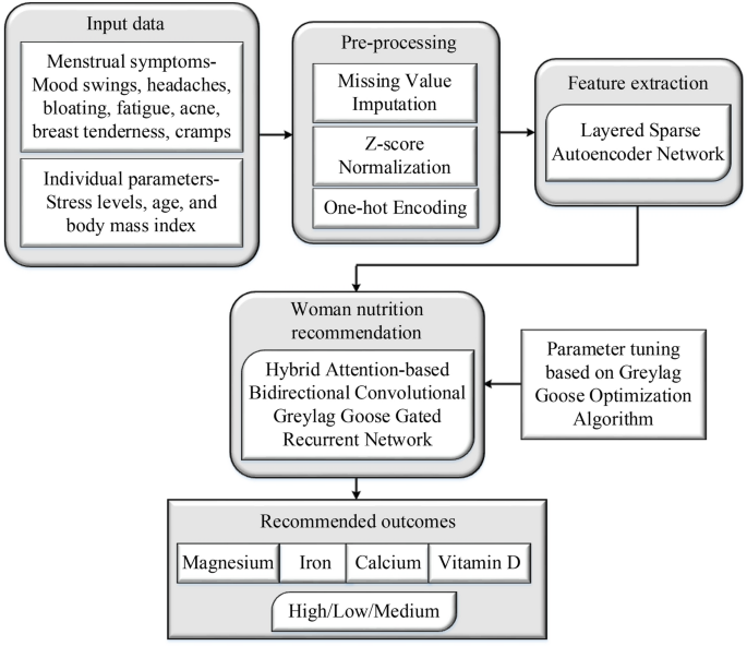
This section discusses a novel OdriHDL model to recommend healthy nutrition for women during the menstrual cycle. The main intention of a proposed OdriHDL model is to analyze complex patterns and offer accurate and individualized advice that enhances menstrual health and overall well-being. Pre-processing is the initial stage where the input data, which comprises mood swings, headaches, bloating, fatigue, acne, breast tenderness, and cramps, as well as personal health information such as stress level, BMI, and age, are pre-processed using Missing Value Imputation, Z-score Normalization, and One-hot Encoding. After that, feature extraction is carried out using a Layered Sparse Autoencoder Network (LSAENet) to extract significant features that support understanding the relationship between nutrient needs and menstrual symptoms. Then, based on the extracted features, a nutrient recommendation is accomplished using the Hybrid Attention-based Bidirectional Convolutional Greylag Goose Gated Recurrent Network (HABi-ConGRNet). To enhance the classification performance, the hyper-parameter of the classification model is tuned using Greylag Goose Optimization Algorithm (GGOA). As a result, the proposed model classifies the level of nutrients (e.g., magnesium, iron, calcium, magnesium, and vitamin D) into categories such as moderate, low, or high.
Figure 1 presents the block diagram of the OdriHDL model, which showcases the flow of data through different stages, including pre-processing, feature extraction, and nutrition recommendation. This architecture effectively captures complex patterns in input data associated to women’s nutritional needs during their menstrual cycle. The incorporation of these steps provides data quality improvement and extraction of significant features as well as improves the model’s overall performance in offering personalized recommendations.

Block diagram of OdriHDL model.
Pre-processing
Data pre-processing is essential to construct a reliable and stable system before DL methods are used in the model. Some data pre-processing operations are carried out to make sure the dataset is clean and prepared for model training. For women’s health nutrition recommendations during the menstrual cycle, the proposed work has discovered missing values and utilized the data imputation approach to replace the missing values. Z-score normalization approaches have been used to identify and replace outliers. Categorical features such as symptoms and the menstrual cycle phase (e.g., menstrual, luteal, follicular, ovulation) are converted into numerical values by using one-hot encoding.
Missing value imputation
The proposed method uses k-nearest neighbors (kNN) to impute the missing values. kNN employs the distance between the sample vectors in the dataset’s space in order to impute the missing data. It deliberates the (k) nearest samples that take the feature observed for each missing feature and averages their values with respect to numerical data. The most frequent class of the kNN is the outcome for categorical data. Given a sample (s(x,y,0)) and its (k) nearest neighbors (N_{k} = { { x_{j} ,y_{j} ,1)|j = 1,2,…,k}), we define:
As there are only binary values, (Z) can only be either (1) or (0), and (1(y_{j} = Z)) resembles a function that returns (0) when ((y_{j} = Z)) and else returns (0). The Euclidean is the metric utilized to compute the distance between two points (q) and (r):
where (p) characterizes the number of variables for each data point.
Z-score normalization
Before applying any models, it is crucial to scale numerical features since scaling is mandatory for various methods, including deep learning. There are various scaling techniques, and in this proposed method a Z-score normalization, also known as zero-mean normalization, has been applied. The mean and standard deviation are utilized to normalize the values for a feature. The expression of Z-score normalization can be given as:
where (Z) indicates the Z-score value, (y) signifies the feature value, (nu) represents the mean value and (chi) states the standard deviation.
One-hot encoding
Models require the conversion of non-numerical features, such as categorical values, into numerical values to enhance the efficiency of model training. To convert the categorical features into one-dimensional binary code vectors, which represent the total number of attributes in the category feature, a one-hot-encoding technique is employed.
Layered sparse autoencoder network
Feature extraction is a process that encompasses identifying and extracting the substantial features that support the recommendation of healthy nutrition for women during their menstrual cycle. An autoencoder (AE)38 is a neural network architecture modeled to learn latent features (compressed representations) of data by reconstructing the input data at the output stage. It comprises two parts, such as an encoder that maps the input into latent space and a decoder that intends for patterns in the lower-dimensional latent space. By imposing sparsity on the hidden units, a sparse AE enhances the efficiency of extracting significant features. In the proposed OdriHDL model, feature extraction is carried out using the Layered Sparse Autoencoder Network (LSAENet) to extract significant features that support the realization of the relationship between nutrient needs and menstrual symptoms. A neural network comprised of several sparse AEs associated end to end is termed a LSAENet. To acquire input data’s high-level feature representations, the output of the sparse self-encoder’s previous layer is passed into the subsequent layer of the self-encoder. Figure 2 illustrates the construction of LSAENet neural network for feature extraction. The output of each layer serves as the input of the next layer. This allows the extraction of higher-level feature representations from the input data. The LSAENet layers are sequentially trained by utilizing the greedy layer-wise pre-training technique39 to obtain the optimal connection weights as well as bias values of the overall sparse AE network layers.

Structure of LSAENet.
Then, to acquire the best parameter model, the LSAENet is fine-tuned by means of an error back-propagation approach until the error function results between the output and input data meet the expected requirements.
For error function (K_{sparse} (omega ,bi)):
Thereby, the weight and bias update process is given as follows:
where (omega) indicates the weight connection between AE layers, (bi) resembles the bias associated with neurons in AE, (mu) resembles the update learning rate, (Y(p)) and (Z(p)) resembles the (p{th}) original vector and its resultant reconstruction vector. Besides, (omega_{jk}^{l}) designates the weight connecting (j{th}) neuron preceding layer to (k{th}) neuron of present layer in (l{th}) layer of LSAENet, (p_{s}) indicates the output of (s{th}) neuron, and (bi^{s}) signifies the bias associated with (s{th}) neuron in the neural network layer.
Different learning rates are used for various parameters, like lowering the update frequency for uncommon features, since the LSAENet network has sparse restrictions. Nonetheless, the majority of popular conventional gradient descent algorithms, such as mini-batch gradient descent and stochastic gradient descent, engage the similar learning rate for every parameter of network that require updating. This makes it challenging to choose an appropriate learning rate and quickly influence at a local minimum. Consequently, an adaptive moment estimation (Adam) gradient descent approach is used to perform dynamic adaptive adjustment of various parameters for training LSAENet. By computing the gradient 1st order moment estimate (n_{u}) and 2nd -order moment estimate (V_{u}), as indicated in formula (8–10), the Adam algorithm allows for the dynamic adjustment of various parameters. Here, (delta_{1}) and (delta_{2}) represent the first- and second-order exponential damping decrements, respectively. The parameters gradient at timestep (u) in the loss function (K_{sparse} (omega ,bi)) is signified by (h_{u}).
where indicates the gradient operation corresponding to the parameter, implies the gradient of loss, and specifies the error function computed at the parameter (weight or bias) (phi) from the preceding iteration (u – 1).
The bias-corrected for (n_{u}) and (V_{u}) can be given as:
Update parameters:
where (zeta) represents the update stepsize, and (psi) indicates a small constant to avoid the denominator to be 0.
Hybrid attention-based bidirectional convolutional Greylag goose gated recurrent network
After extracting the features, the proposed OdriHDL model has employed a Hybrid Attention-based Bidirectional Convolutional Greylag Goose Gated Recurrent Network (HABi-ConGRNet) for women’s health nutrition recommendations during the menstrual cycle. HABi-ConGRNet combines CNN, bidirectional GRU (BiGRU), cross attention mechanism (CrAM) and Greylag Goose Optimization Algorithm (GGOA). The CNN acquires spatial correlations between health metrics and nutrients after feature extraction, which identifies critical features, including age, cycle stages, health conditions, etc. It recognizes patterns in nutritional requirements, like the demand for iron deficit during menstruation or calcium during the luteal phase. Then, the sequential nature of the menstrual cycle is handled by the BiGRU, which acquires knowledge of the time-dependent changes in nutrient needs across various phases. BiGRU supports in predicting which nutrients are most important at particular times in the cycle by identifying these variations. Consequently, the CrAM dynamically assigns a higher priority to specific features, like iron during menstruation and magnesium during other phases etc. This ensures that recommendations are highly associated with the current stage and condition. By combining this technique, the hybrid model effectively learns both the cyclical patterns and specific nutritional priorities in order to offer customized health nutrition advice that changes according to the changing needs of users during the menstrual cycle.
Figure 3 indicates the architecture of HABi-ConGRNet model. It resembles the sequential flow of sequential features through different components, including the input layer, multiple convolution layer, max pooling layer, and BiGRU layer, which acquires temporal dependencies in the data. In addition, the cross-attention mechanism (CrAM) is incorporated to prioritize important features. This permits the model to dynamically adjust nutritional recommendations depending on the specific stage of the menstrual cycle and individual health metrics.

Architecture of HABi-ConGRNet model.
Convolutional neural network
One of the representative algorithms of DL is considered as CNN40. It is a deep-structured feedforward neural network that includes convolution computation. The biological visual perception system was imitated in the construction of CNN. The sparsity of connections between layers and sharing the hidden layer’s convolution kernel parameter allows the CNN to extract features with minimal computation. The input layer, convolutional layer, pooling layer, and fully connected (FC) layer are composed in the entire structure of CNN. In the input layer, the extracted features are given as input. The convolutional layer applies a convolution computation to the input by convolutional kernel for obtaining feature map. Usually, several convolution kernels are utilized to perform feature extraction to better utilize convolution kernels. The combination encompassing (Z) convolution kernels is signified by ([Q_{1} ,Q_{2} ,Q_{3} ,….,Q_{Z} ]), where (Q_{Z}) resembles (Z{th}) convolution kernel size, or the convolution kernel window’s longitudinal dimension. The vector dimension of the feature vector is equal to the horizontal convolution kernel window size.
There will be (Z) feature map vectors after calculating (Z) convolution kernels. The convolution window size is given as (I). The convolution kernel is applied to carry out the convolution operation on the input windows (y_{1}^{H} ,y_{2}^{H} ,y_{3}^{H} ,…,y_{p – H + 1}^{p}) to extract the local features. Assume that the input (D) comprises of (p) feature vectors, (y_{1} ,y_{2} ,y_{3} ,….,y_{p}), the convolutional layer’s function can be written as
where (g( * )) signifies the nonlinear function, (H) resembles the dimension of the convolution kernel, (B) specifies the bias vector and (X) indicates the weight matrix. The combination of vectors is represented by the symbol (y_{j:j + H – 1}).
After the extraction of the convolution kernel, the eigenvector (z) is obtained as:
Following the convolution operation, each eigenvector is exposed to pooling processing by means of the pooling layer. The multidimensional vector is transformed into a value after pooling, which is utilized as a pooled vector element. The sequence output from the convolutional layer is passed into the pooling layer using the maximum pooling approach, which is used by the pooling layer. The largest element in the series (z_{1} ,z_{2} ,z_{3} ,….,z_{p – H + 1}) will be elected by the maximum pooling method, which will finally provide a new vector (z):
Bidirectional gated recurrent unit
A type of RNN is deliberated as GRU. Like LSTM, GRU is also regarded as a solution for long-term memory and gradients in backpropagation. RNNs execute recursion in the evolutionary sequence direction with input sequential data, and here, every neuron is connected in a chain. Neurons can concurrently receive information from other neurons and their own historical instants owing to the inclusion of the hidden layer’s cyclic factors. Thereby, RNN has parameter sharing and memory sharing. Besides, RNN performs better while learning nonlinear features from serial data. LSTM is presented as a solution to the disappearing RNN gradient problem and its incompetence in learning long-term historical features. LSTM can learn correlation data between short-term and long-term sequential data. Later, GRU was established as a solution to the issue of LSTM with a slower convergence rate and excessive parameters. A variant of LSTM with fewer parameters is known as GRU, which exhibits faster convergence performance without losing the greater learning ability of LSTM. The internal components of GRU include the update gate and reset gate.
The structure of BiGRU is displayed in Fig. 4. It highlights its internal components comprising update gate and reset gate. This structure permits the BiGRU to effectively manage information flow by determining which feature to discard or retain. Thereby, addressing the challenges of long-term dependencies in sequential data. In contrast to LSTM, GRU exchanges the forgetting gate and input gate of an LSTM with an update gate. The update gate specifies the impact of hidden layer neurons’ output data from a preceding moment on the neurons in the current hidden layer. A higher updating gate value resembles to a higher degree of influence. In contrast to LSTM, GRU exchanges the forgetting gate and input gate of an LSTM with an update gate. The update gate specifies the impact of hidden layer neurons’ output data from a preceding moment on the neurons in the current hidden layer. A higher updating gate value resembles a higher degree of influence. The neglect degree of neuron output in a hidden layer at preceding is characterized by the resetting gate. The following formula can be employed to define the hidden layer unit (B):
where (delta) indicates the Sigmoid function, (tanh) specifies the hyperbolic tangent function, and (Z_{u}) and (R_{u}) specify the updating and resetting gates. (w_{R}), (v_{R}), (w_{Z}), (v_{Z}), and (v) signify all the matrices of training parameter. The resetting gate (R_{u}), the input (Y_{u}) at the current instant, the output (H_{u – 1}) of the hidden layer neuron at the preceding moment, and the training parameter matrices (v) and (u) work together to establish the candidate activation state (tilde{H}_{u}) at the present moment.

Structure of BiGRU.
To learn the deep features of women’s nutrition recommendations, the BiGRU network is better for learning the relationship between current, past, and future influencing factors41. It is computed as
and (B_{2}^{prime}) are computed using
The hidden layer value (S_{u}) in the forward calculation is associated to (S_{u – 1}). The value of hidden layer (S_{u}) in the reverse computation is associated to (S_{u – 1}). The sum of the reverse and forward computations governs the final result. The calculation procedure of bidirectional RNN is given as follows:
The cross-entropy (CE) loss function is employed for the classification problem in the neural network42. The provided metaheuristic algorithm tunes the hyperparameters of the classification model by minimizing the loss function.
Cross-attention mechanism
The attention mechanism (AM) is modeled to minimize the intervention of inappropriate data while getting the most significant information for recommending health nutrients and assisting in making the best possible decisions. The AM performs well in two ways: first, it automatically ascertains the local data that needs to be concentrated in the global input. Second, it gives more processing power to task-critical computations. AM is frequently used to improve local information features because of these two benefits. Additionally, the task objective and the attention region are different. The most important information is used efficiently when local information is gathered. The output of the attention network is stated as follows:
where (Z_{u}) characterizes the output of AM at an instant (u), (g) specifies the dense layer, (Z_{u – 1}) implies the output of AM at time (u – 1), and (m_{u – 1}) designates the label at moment (u – 1).
where (D_{u}) characterizes the output of succeeding phase, (i_{k}) implies the (k{th}) input of AM, and (b_{uk}) designates the attention weight,.
where (h) is employed to compute the extent of association between (Z_{u – 1}) and (i_{k}), and (b_{uk}) designates the degree to which the current AM is allied and (k{th}) input. More attention is engrossed on the component when the extent of association is greater.
Cross-attention
The conventional AM, which a one-way AM that allocated weight to attention in only one direction, lost a number of distinctive variables. The summing of the weight matrix via elements and the weight maximization strategy are the two tandem weight allocation techniques used by the HABi-ConGRNet. It also utilizes the cross-attention mechanism (CrAM). The weight coefficients are first calculated in the vertical and horizontal directions using the CrAM. The structure of CrAM is provided in Fig. 5. The CrAM allocates attention weights in both vertical and horizontal directions. By obtaining the most representative features, this dual-directional method progresses feature extraction. The mechanism improves the model’s performance by using weight addition and maximization methods. The schematic demonstrates how the weights are computed and applied to the input data. This mechanism reduces information loss and guarantees effective feature mining.

Structure of CrAM.
The resulting element weights are then increased in two perpendicular directions to strengthen the features, and a maximizing technique is employed to get maximum weight coefficients. As a result, the combined result of two methods has been gained. Weights are multiplied and maximized using the expression below.
where (Z_{1}) designates the weight coefficient of vertical AM, (Z_{2}) describes the weight coefficient of horizontal AM, (Add) signifies the weight coefficients summation and (Max) specifies the maximization of weight coefficients. CrAM in HABi-ConGRNet gives weight values to the feature map’s output by BiGRU from two mutually perpendicular dimensions. Next, it fuses those feature maps with the original feature map by maximizing and summing the weight values, which specifies the major features and optimizes the computational resources.
Hyper-parameter tuning
Hyper-parameter tuning is deliberated as choosing the optimal values for parameters in the classification model of the proposed OdriHDL approach. A Greylag Goose Optimization Algorithm (GGOA) is used in the proposed OdriHDL approach to tuning the hyper-parameters for enhancing the classification performance. GGOA takes ideas from the dynamic characteristics of geese. It starts by randomly building individuals, each of which characterizes a potential solution for a certain issue. Then, these individuals are split up into groups for exploration and exploitation, with the size of each group changing according to how successfully the optimal solution is performed. This prevents the algorithm from becoming stuck in local optima and tends to an efficient search of the solution space. For hyper-parameter tuning, the individual geese are considered hyper-parameters, and the optimal parameter values are considered as the best solution.
The exploration operation of GGOA is concerned with locating promising regions in the search space and circumventing local optima stagnation by moving in the direction of the optimal solution. This is achieved by using specific equations to alter the position of the agents iteratively. The primary equation of GGOA for updating agent location is given as:
where (Y(u)) designates the position of the agent at iteration (u), and (Y^{prime} (u)) designates the position of the best solution (leader). During iterations, the GGOA utilizes the following equations to update vectors (B) and (D), which are designated as (B = 2b.s_{1} – b) and (D = 2.s_{2}), respectively. The parameter (b) varies linearly from 2 to 0. (s_{1}) and (s_{2}) are randomly altering values within ([0,1][0,1]).
The following equation, which considers three randomly chosen search agents (paddings), designated as (Y_{Paddle,,1}), (Y_{Paddle,,2}), and (Y_{Paddle,,3}), is incorporated into the algorithm to further enhance exploration:
where (W_{,1}), (W_{,2}), and (W_{,3}) are updated within ([0,2]), and (Z) is minimized exponentially depending on (Z = 1 – left( {{u mathord{left/ {vphantom {u {u_{Max} }}} right. kern-0pt} {u_{Max} }}} right)^{2}), where (u_{Max}) represents the maximum number of iterations.
In the second updating stage, when (s_{,3} ge 0.5), the values of (b) and vector (B) are decreased:
where, (W_{,4}) updates within ([0,2]), (m) specifies the random number in ([ – 1,1]), (s_{4}) and (s_{5}) update within [0,1], and (c) indicates a constant.
The exploitative dimension of GGOA is devoted to improving upon previously developed solutions depending on the fitness (Mean Square Error (MSE)). Two distinct tactics are used to achieve the exploitation objectives. These strategies work together to enhance the overall quality of the solution.
-
1.
Moving in the direction of best solution: In order to direct individuals ((Y_{nonsentry,,1} )) toward the predicted prey position, the algorithm utilizes the following equation, which is guided by three sentry solutions ((Y_{sentry,,1} ,Y_{sentry,,2}) and (Y_{sentry,,3})).
$$Y_{1} = Y_{sentry,,1} – B_{1} .left| {D_{1} .,Y_{sentry,,1} – Y} right|$$(38)$$Y_{2} = Y_{sentry,,2} – B_{2} .left| {D_{1} .,Y_{sentry,,2} – Y} right|$$(39)$$Y_{3} = Y_{sentry,,3} – B_{3} .left| {D_{1} .,Y_{sentry,,3} – Y} right|$$(40)where (D_{,1}), (D_{,2}) and (D_{,3}) are calculated as (D = 2s_{2}), and (B_{,1}), (B_{,2}) and (B_{,3}) are computed as (B = 2b,.,s_{1} – b). The average of three solutions, (Y_{,1} ,,,Y_{,2}) and (Y_{,3}), is used to define the updated locations for the population, (Y(u + 1)) as follows:
$$Y(u + 1) = frac{1}{3}sumlimits_{j = 1}^{3} {Y_{j} }$$(41) -
2.
Searching the area around optimal solution: In this tactic, individuals look for improvements in areas close to the optimal solution. The equation for updating a position is offered by:
$$Y(u + 1) = Y(u) + E(1 + a) * W * (Y – Y_{fok} )$$(42)where (W) represents an additional exploration parameter, (E) resembles a constant, (a) states a parameter computed by the number of iterations, and (Y_{fok}) indicates the optimal response (leader).
These techniques move individuals’ positions toward more promising areas of the search space, allowing the GGOA to enhance solutions continuously. The pseudocode of GGOA for optimal parameter tuning is offered in Algorithm 1.

Pseudocode of GGOA for hyper-parameter tuning
Results and discussion
This subdivision provides the results of using the OdriHDL model to recommend women’s health nutrition. The OdriHDL model is implemented using python programming language. Several existing techniques, such as RNN, CNN with LSTM (CNN-LSTM), CNN with BiLSTM (CNN-BiLSTM), and attention GRU have been taken into account in order to calculate and analyze the classification performance of OdriHDL model. The system configuration of proposed OdriHDL model is given in Table 2. An Intel CoreI i5-4667S CPU running at 4.10 GHz offers strong processing power to manage complex DL operations. It has a 64-bit operating system, which permits efficient memory management and the capability to utilize more RAM. Besides, the system has 16.0 GB of installed RAM which improves the model’s performance during the training and testing stage. This ensures quick data processing and smooth operation.
Table 3 shows the OdriHDL model’s hyperparameters. It includes a maximum of 100 epochs for training, with a learning rate set at 0.01 to control the step size during optimization. The model utilizes GGOA as an optimizer and employs a mini-batch size of 32 for efficient training data processing. The loss function employed is cross-entropy (CE), with a dropout rate of 0.5 to prevent overfitting. The collected data is divided into 20% for testing and 80% for training to assess the model performance.
The OdriHDL model provides real-time and personalized nutrition suggestions to control symptoms and improves health during the menstrual cycle. In addition, the following sections provide the data collection, performance evaluation, and assessment metrics for the OdriHDL model for women’s nutrition recommendations during the menstrual cycle.
Data collection
For experimentation, the real-time data was collected through in-depth discussions with consultants in menstrual health and nutrition. The mapping of particular nutrient recommendations to symptoms (such as intense cramps etc.) was aided by expert assistance. The collected data comprises of 2000 samples that are used for deep learning model training. Menstrual symptoms like mood swings, headaches, bloating, fatigue, acne, breast tenderness, and cramps, and individual parameters like stress levels, age, and Body Mass Index (BMI) are considered as inputs. The predicted nutrient recommendations for iron, magnesium, calcium, and vitamin D are moderate, low or high. For each data, unique identifier, BMI (18.5–30.5), age of persons from 18 to 50, level of stress from 0 (no stress) to 3 (severe stress), menstrual cycle day 1 to 28, cycle phase considered as follicular, menstruation, luteal or ovulation are considered. In addition, the menstrual cycle-related symptoms such as mood swings, headaches, bloating, fatigue, acne, breast tenderness, and cramps, are rated from 0 to 3 in which 0 indicates no symptoms, 1 states low, 2 represents medium and 3 resembles severe/high. Based on the input, the predicted nutrition includes the intake of calcium (mg/day), iron (mg/day), magnesium (mg/day), and vitamin D (IU/day). Also, these nutrition needs are classified as moderate, low, or high.
For iron, class low indicates to a low requirement of 0–10 mg daily, class moderate resembles 10–18 mg, and class high suggests the need for more than 18 mg. For calcium, the class low indicates the intake of 0–500 mg daily, moderate denotes the intake of 500–1000 mg, and high denotes more than 1000 mg of need. Similarly, for magnesium, low resembles to a low intake of 0–200 mg, moderate resembles an intake of 200–400 mg, and high specifies the demand exceeding 400 mg. Lastly, for vitamin D, low specifies the intake of 0–1000 IU per day, moderate represents the intake between 1000 and 2000 IU, and high defines the intake of more than 2000 IU. Utilizing this collected data, the proposed OdriHDL model is trained to recommend women’s nutrition needs for magnesium, calcium, iron, and vitamin D based on their menstrual phase, symptoms, and personal health information.
Performance metrics
The OdriHDL model for women’s nutrition recommendations during menstrual cycles is evaluated using various measures, including accuracy, precision, recall, specificity, f1-score, R square, mean absolute error (MAE), R square, mean square error (MSE), and root mean square error (RMSE). The mathematical formulae for computing these evaluation measures are given below.
where ({rm K}_{tn}) symbolizes true negative, ({rm K}_{tp}) designates true positive, ({rm K}_{fp}) suggests false positive and ({rm K}_{fn}) characterizes false negative.(y(p)) and (y^{primeprimeprime}(p)) state the actual and predicted value. Besides, (y{}_{j}) indicates the actual value of (j{th}) observation, (y^{prime} {}_{j}) designates the predicted value of (j{th}) observation and (overline{y}) resembles the mean of all (y{}_{j}) values.
Performance evaluation in terms of evaluation metrics
The simulation outcomes of the OdriHDL model for women’s nutrition recommendation during the menstrual cycle have been assessed in this subsection. The results of the OdriHDL model are contrasted with those of popular deep learning architectures, including RNN, CNN-LSTM, CNN-BiLSTM, and attention GRU. The accuracy comparison between OdriHDL model and existing architectures for recommending women’s nutrition is validated in Fig. 6. The OdriHDL model’s robustness prediction is shown in graphical form. The accuracy rate achieved by the OdriHDL model is about 97.52%, which enhances women’s nutrition recommendation process more effectively. On the other hand, the accuracy value accomplished by the prevailing classifiers for women’s nutrition recommendation is minimized owing to multiple complexities. RNN performs incorrectly due to difficulty in interpretation and is prone to gradient disappearance issues. CNN-LSTM and CNN-BiLSTM undertake certain drawbacks, such as difficulty in learning over long sequences, limited memory capacity, and exhibit overfitting issues. Besides, the gating technique in GRU aids in addressing the vanishing gradient issue, nonetheless, it cannot be more efficient. The combination of LSAENet and HABi-ConGRNet offer a novel remedy for the problems currently arising in OdriHDL model for recommending women nutrition.

Evaluation of model performance using accuracy metric.
Figure 7 shows the comparative analysis of precision for women’s nutrition recommendations during the menstrual cycle using OdriHDL and existing models. Due to the obtainability of the best HABi-ConGRNet for recommending women’s nutrition, the OdriHDL has improved its precision rate over existing RNN, CNN-LSTM, CNN-BiLSTM, and attention GRU models. Among the existing architectures, attention GRU has gained the highest precision closer to the OdriHDL model, whereas RNN has obtained a lower precision value. As a result, OdriHDL model is renowned for precisely measuring the rate of wrong values and efficaciously determining the classes. The recall performance of OdriHDL model and the prevailing models for women’s nutrition recommendation is shown in Fig. 8. The recall performance in OdriHDL is compared to existing methods to demonstrate how well the model can recommend nutrition for women during the menstrual cycle. Similar to accuracy and precision, the OdriHDL model outperformed the existing methods regarding recall performance, as recognized by the graphical depiction. The recall value obtained by OdriHDL model is 96.91%. This is because the network incorporates a robust classifier as well as efficient tuning of parameters through GGOA, which improve the recall value.

Evaluation of model performance using precision metric.

Evaluation of model performance using recall metric.
Another significant metric used for recommending women nutrition during menstrual cycle is the specificity. For nutrition recommendation, a model with a higher specificity is said to be superior. Figure 9 presents the evaluation of specificity for the proposed OdriHDL model and the dominant classifiers for women nutrition recommendation. The graphical representation makes it evident that, in terms of the specificity value, the proposed OdriHDL model has done better than other models like RNN, CNN-LSTM, CNN-BiLSTM, and attention GRU. The maximum specificity value obtained by OdriHDL model is 97.41%. Because of the extraction of useful features using LSAENet, the OdriHDL model recommends women nutrition more correctly.

Evaluation of model performance using specificity metric.
The assessment of the f1-score obtained by the OdriHDL model and the current classifiers for women’s nutrition recommendations during the menstrual cycle is shown in Fig. 10. For a given input, the OdriHDL model can accurately and effectively classify the required nutrition for women during the menstrual cycle. Furthermore, the f1-score states the precise positive rates ensuing from multiple distinctiveness mappings using parametric input data. Additionally, it is clear from the graphical depiction that the OdriHDL model has outperformed other existing methods such as RNN, CNN-LSTM, CNN-BiLSTM, and attention GRU regarding the f1-score value due to selecting an appropriate classifier. The OdriHDL model’s f1-score outperforms the existing classifiers by roughly 97.36%. As a result, the OdriHDL model is more accurate in defining the classes of automated women’s nutrition recommendations.

Evaluation of model performance using f1-score metric.
Besides, MAE, MSE, and RMSE are substantial metrics associated to discovering the error measures. For women’s nutrition recommendations during the menstrual cycle, the OdriHDL model is considered superior if the value of error measures such as MAE, MSE, and RMSE is lower. Figure 11 shows the MSE analysis by the OdriHDL model and the current classifiers for recommending women’s nutrition during the menstrual cycle. In the graphical depiction, the OdriHDL model has gained a lower MAE value than the prevailing one. The comparative study of MAE for recommending women’s nutrition during the menstrual cycle using OdriHDL and existing classifiers is depicted in Fig. 12. The OdriHDL model has attained the least MAE related with RNN, CNN-LSTM, CNN-BiLSTM, and attention GRU models because of HABi-ConGRNet. The prevailing models have attained greater MAE values for nutrition recommendation. The OdriHDL model has obtained a minimum MAE of 0.17. This shows the error reduction ability of the proposed model. Similarly, Fig. 13 validates the RMSE with OdriHDL and existing classifiers. On noticing the graphical illustration, the OdriHDL model has accomplished supreme RMSE values of 0.5385 and is lower than the existing models. The prevailing methods have attained greater RMSE values than OdriHDL model since the classification of women nutrition is not better. Overall, it is implicit that the OdriHDL has suitably reduced the error rates in women nutrition recommendation.

Evaluation of model performance using MSE metric.

Evaluation of model performance using MAE metric.

Evaluation of model performance using RMSE metric.
The R square metric is reflected as one of the most suitable performances recommending women’s nutrition during the menstrual cycle. The percentage of variance in determined women’s nutrition values accounted by the model is normally quantified as R square. In women’s nutrition recommendation, R square assesses how well the OdriHDL model represents the accuracy of women nutrition level classification and the variation between actual and expected values. Figure 14 characterizes the obtained R square value of OdriHDL model and existing RNN, CNN-LSTM, CNN-BiLSTM, and attention GRU for women’s nutrition recommendation. If the R square value is greater and close to 1, it states that the OdriHDL model is more reliable and accurate for women nutrition recommendations. On the other hand, a smaller R square value suggests the variability in the data cannot be captured by OdriHDL model. The graphical depiction shows that the OdriHDL model has a higher R square value of 96%, which is better than the existing methods.

Evaluation of model performance using R square metric.
Table 4 investigates the proposed OdriHDL model and existing models. such as CNN-LSTM, RNN, CNN-BiLSTM, and attention GRU. Here, significant measures such as accuracy, recall, precision, specificity, F1-score, MSE, MAE, RMSE, and R-squared values are used for assessing. In terms of accuracy and precision, the OdriHDL model performs better than the existing model, accomplishing 97.52% and 97.82%. This exemplifies how well the model can categorize women’s nutritional needs during their menstrual cycle.
Performance evaluation in terms of accuracy-loss
This section uses training and testing data to assess the accuracy and loss performance of the OdriHDL for recommending women’s nutrition during the menstrual cycle. The training and testing accuracy of OdriHDL model for women’s nutrition recommendation is exposed in Fig. 15. The training and testing accuracy of OdriHDL model is evaluated and revealed in the graph by changing the epoch size from 0 to 100. As the value of the epoch increases, the OdriHDL model’s training accuracy is improved. Accordingly, testing and training accuracy are nearly comparable in the graphical illustration. The similarity in training and testing curves describes the ability of the nearly model to influence the test samples for recommending women’s nutrition.

Training and testing accuracy of OdriHDL model.
Similarly, the training and testing losses gotten by the OdriHDL model are exhibited in Fig. 16. The loss during the testing phase exposes that the OdriHDL methodology for women’s nutrition recommendation incurs low loss. The HABi-ConGRNet model produced higher results for testing and training data. Besides, the OdriHDL model decreased overfitting and increased convergence. The difference between the training and testing curves decreases with increasing epochs, which is expected to improve women’s nutrition recommendations during the menstrual cycle. The use of GGOA for parameter change condenses error values and supports performance enhancement.

Training and testing loss of OdriHDL model.
Convergence analysis
The effectiveness of GGOA in proposed OdriHDL model is verified through convergence analysis. For parameter adjustment, the convergence curve more clearly displays GGOA’s exploratory and exploitative behavior. The convergence curve under various optimization strategies is shown in Fig. 17. Here, the suggested GGOA and parrot optimization algorithm are contrasted. Although GGOA converges a bit longer in the first iteration, it obtains superior final values of the objective function. This helps to avoid the local optimum problem and improve the exploitation ability. Furthermore, by greatly enhancing fitness performance and reducing classification error, the GGOA enhances classification performance. Additionally, the suggested GGOA takes less iterations than parrot optimization, as demonstrated by the graphical representation. Furthermore, throughout the search iteration, the GGOA is successful in striking a balance between exploration and exploitation.

Convergence analysis.
Hypothesis and limitation
Clinical trials and observational research have historically been the backbones of the nutrition sector, but the introduction of AI has replaced them. These technologies, which include data analysis, DL, and ML, have the capacity to find patterns, produce significant information, and reveal intricate relationships in data. In this section, the OdriHDL model designed to offer personalized nutrition recommendations is discussed. The OdriHDL model leverages HABi-ConGRNet to assess complex patterns in nutritional needs by considering individual health metrics and menstrual symptoms. The model includes comprehensive data pre-processing, feature extraction based on LSAENet, and a robust classification approach to improve recommendation accuracy. With a 97.52% accuracy rate, the quantitative outcomes demonstrate its capability to effectively classify and recommend essential nutrition, outperforming existing RNN, CNN-LSTM, CNN-BiLSTM, and attention GRU models, which have attained lower accuracy rates ranging from 85 to 92%. The recall of 96.91% and precision of 97.82% highlight the model’s reliability in accurately determining the nutritional needs of women. Additionally, to further determine the model’s superiority, the proposed OdriHDL is compared with state-of-the-art methods in Table 5. In the table, the existing LSTM, which is applied for patient diet recommendation has attained better performance but it has occurred overfitting process and less convergence. Another method K-clique integrated GRU classifier has attained less accuracy. However, the proposed OdriHDL model has attained better accuracy as well as it solves the overfitting issues.
This proves the potential of OdriHDL model for practical application in health technology. The primary advantage of OdriHDL model is its incorporation of an advanced feature extraction model through LSAENet, which boosts the model to capture complex relationships between nutritional requirements and menstrual symptoms. In addition, the usage of HABi-ConGRNet permits an understanding of data, tending to enhanced classification performance. The optimization of the model also contributes to reduced training time and faster convergence, making it efficient for real-world applications. Despite the improvements, the proposed model poses certain limitations. The reliance of specific data can limit the model’s generalizability, as it may not account for diverse experiences and nutritional needs. Besides, the complexity of architecture creates challenges in terms of interpretability and ease of implementation in everyday settings even showing promise in accuracy.
Conclusion
This paper contributes to a new OdriHDL model for recommending women’s nutrition during the menstrual cycle. The OdriHDL model performed exceptionally well in classifying women’s nutrition into levels of calcium, magnesium, iron, and vitamin D due to the use of a hybrid DL method. Numerous features such as the symptoms related to the menstrual cycle and personal attributes extracted through LSAENet in the OdriHDL model, help HABi-ConGRNet classifier to improve performance. Furthermore, the OdriHDL model is optimized using a GGOA for parameter tuning, accelerating the training process with few iterations. The proposed OdriHDL model is compared and tested against existing models such as RNN, CNN-LSTM, CNN-BiLSTM, and attention GRU, demonstrating accurate performance with little complexity. The proposed OdriHDL model is simulated using the Python platform and exhibits a variety of performance indicators. The OdriHDL model has attained a remarkable accuracy of 97.52%, with 97.82% precision, 96.91% recall, 97.41% specificity, and 97.36% f1-score. These findings demonstrate its superior capability to offer personalized nutrition recommendations. Further, the variation in the outcomes of OdriHDL model when compared to existing methods is mainly due to ability to extract vital features using LSAENet, which minimizes the complexities of women’s nutritional needs during the menstrual cycle. Additionally, the incorporation of advanced DL model improves the model’s accuracy and minimizes the overfitting problems perceived in the existing methods. Even if the performance of the proposed OdriHDL model is remarkable for recommending women’s nutrition, further development of learning architecture and optimization can progress their efficiency, scalability, and accuracy.
Data availability
The following Datasets available for references (1) Menstrual-Health-Awareness-Dataset—https://huggingface.co/datasets/gjyotk/Menstrual-Health-Awareness-Dataset/viewer/default/train?p=5 (2) Menstrual cycle—https://www.kaggle.com/datasets/nikitabisht/menstrual-cycle-data (3) Mood swing—https://www.kaggle.com/code/swapnilbhowmik/student-mental-health-prediction-analysis (4) Menstruation symptoms—https://helloclue.com/articles/emotions/mood-changes-and-the-menstrual-cycle. (5) Nutrition—https://www.kaggle.com/code/fernandodiazc/bellabeat-case-study-with-rhttps://www.kaggle.com/code/laurapasqualette/bellabeat-casestudyjan2024 (6) https://www.kaggle.com/code/harrietikpea/bella-beat-data-analysis-in-r Extracted Dataset from the above Available Datasets (1) menstrual_symptoms_dataset 1.xlsx (Upload as Supplementary material) (2) Women nutrition recommendation data 2.csv (Upload as Supplementary material).
References
-
Itriyeva, K. The normal menstrual cycle. Curr. Probl. Pediatr. Adolesc. Health Care 52(5), 101183 (2022).
Google Scholar
-
Taim, B. C. et al. The prevalence of menstrual cycle disorders and menstrual cycle-related symptoms in female athletes: A systematic literature review. Sports Med. 53(10), 1963–1984 (2023).
Google Scholar
-
Tucker, J. A. L., McCarthy, S. F., Bornath, D. P. D., Khoja, J. S. & Hazell, T. J. The effect of the menstrual cycle on energy intake: A systematic review and meta-analysis. Nutr. Rev. https://doi.org/10.1093/nutrit/nuae093 (2024).
Google Scholar
-
Roby, P. R., Grimberg, A., Master, C. L. & Arbogast, K. B. Menstrual cycle patterns after concussion in adolescent patients. J. Pediatr. 262, 113349 (2023).
Google Scholar
-
de Assis, F. et al. Menstrual cycle and strength levels in women: A pilot study. Cuadernos de Educación y Desarrollo 16(5), e4197. https://doi.org/10.55905/cuadv16n5-046 (2024).
Google Scholar
-
Cunningham, A. C. et al. Chronicling menstrual cycle patterns across the reproductive lifespan with real-world data. Sci. Rep. https://doi.org/10.1038/s41598-024-60373-3 (2024).
Google Scholar
-
Ju, Q. et al. Regulation of craving training to support healthy food choices under stress: A randomized control trial employing the hierarchical drift-diffusion model. Appl. Psychol. Health Well Being 16(3), 1159–1177 (2024).
Google Scholar
-
Sen, L. C. et al. Food craving, vitamin A, and menstrual disorders: A comprehensive study on university female students. PLOS ONE 19(9), e0310995 (2024).
Google Scholar
-
Bai, M. et al. Hydrolyzed protein formula improves the nutritional tolerance by increasing intestinal development and altering cecal microbiota in low-birth-weight piglets. Front. Nutr. 11, 1439110. https://doi.org/10.3389/fnut.2024.1439110 (2024).
Google Scholar
-
Langan-Evans, C. et al. Hormonal contraceptive use, menstrual cycle characteristics and training/nutrition related profiles of elite, sub-elite and amateur athletes and exercisers: One size is unlikely to fit all. Int. J. Sports Sci. Coach. 19(1), 113–128 (2024).
Google Scholar
-
Pavani, M., Monisha, D. R., Lavanya, B. & Takalkar, A. A. Menstrual pattern amongst adolescent girls: A cross sectional study from Raichur, Karnataka. Int. J. Reprod. Contracept. Obstet. Gynecol. 10(12), 4429. https://doi.org/10.18203/2320-1770.ijrcog20214636 (2021).
Google Scholar
-
Kapoor, R., Sabharwal, M. & Ghosh-Jerath, S. Diet quality, nutritional adequacy and anthropometric status among indigenous women of reproductive age group (15–49 Years) in India: A narrative review. Dietetics 2(1), 1–22 (2022).
Google Scholar
-
Aguree, S., Murray-Kolb, L. E., Diaz, F. & Gernand, A. D. Menstrual cycle-associated changes in micronutrient biomarkers concentration: A prospective cohort study. J. Am. Nutr. Assoc. 42(4), 339–348 (2023).
Google Scholar
-
Feskens, E. J. M. et al. Women’s health: Optimal nutrition throughout the lifecycle. Eur. J. Nutr. 61(S1), 1–23. https://doi.org/10.1007/s00394-022-02915-x (2022).
Google Scholar
-
Thanarajan, T., Alotaibi, Y., Rajendran, S. & Nagappan, K. Improved wolf swarm optimization with deep-learning-based movement analysis and self-regulated human activity recognition. AIMS Math. 8(5), 12520–12539 (2023).
Google Scholar
-
Ko, H., Lee, S., Park, Y. & Choi, A. A survey of recommendation systems: Recommendation models, techniques, and application fields. Electronics 11(1), 141 (2022).
Google Scholar
-
Balasubramaniam, S., Arishma, M. & Dhanaraj, R. K. A comprehensive exploration of artificial intelligence methods for COVID-19 diagnosis. EAI Endorsed Trans. Pervasive Health Technol. https://doi.org/10.4108/eetpht.10.5174 (2024).
Google Scholar
-
Thanarajan, T., Alotaibi, Y., Rajendran, S. & Nagappan, K. Eye-tracking based autism spectrum disorder diagnosis using chaotic butterfly optimization with deep learning model. Comput. Mater. Contin. 76(2), 1995–2013 (2023).
-
Balasubramaniam, S., Nelson, S. G., Arishma, M. & Rajan, A. S. Machine learning based disease and pest detection in agricultural crops. EAI Endorsed Trans. Internet Things https://doi.org/10.4108/eetiot.5049 (2024).
Google Scholar
-
Balasubramaniam, S. & Arishma, M. Prediction of breast cancer using ensemble learning and boosting techniques. In 2024 International Conference on Communication, Computer Sciences and Engineering (IC3SE), 513–519 (IEEE, 2024).
-
Rahman, M. M. et al. Empowering early detection: A web-based machine learning approach for PCOS prediction. Inform. Med. Unlock. 47, 101500. https://doi.org/10.1016/j.imu.2024.101500 (2024).
Google Scholar
-
Chan, L. E. et al. Predicting nutrition and environmental factors associated with female reproductive disorders using a knowledge graph and random forests. Int. J. Med. Inform. 187, 105461 (2024).
Google Scholar
-
Dong, S., Wang, P. & Abbas, K. A survey on deep learning and its applications. Comput. Sci. Rev. 40, 100379 (2021).
Google Scholar
-
Rajesh, T. R., Rajendran, S. & Alharbi, M. Penguin search optimization algorithm with multi-agent reinforcement learning for disease prediction and recommendation model. J. Intell. Fuzzy Syst. 44(5), 8521–8533 (2023).
Google Scholar
-
Balasubramaniam, S., Prasanth, A., Satheesh Kumar, K. & Kavitha, V. Medical image analysis based on deep learning approach for early diagnosis of diseases. In Deep Learning for Smart Healthcare: Trends, Challenges and Applications (eds Murugeswari, K. et al.) 54–75 (Auerbach Publications, 2024).
Google Scholar
-
Fang, H., Zhang, D., Shu, Y. & Guo, G. Deep learning for sequential recommendation: Algorithms, influential factors, and evaluations. ACM Trans. Inform. Syst. (TOIS) 39(1), 1–42 (2020).
Google Scholar
-
Balasubramaniam, S., Seifedine Kadry, K. & Kumar, S. Osprey Gannet optimization enabled CNN based Transfer learning for optic disc detection and cardiovascular risk prediction using retinal fundus images. Biomed. Signal Process. Control 93, 106177. https://doi.org/10.1016/j.bspc.2024.106177 (2024).
Google Scholar
-
Sajindra, H., Thilina Abekoon, J. A. D. C. A. & Jayakody, U. R. A novel deep learning model to predict the soil nutrient levels (N, P, and K) in cabbage cultivation. Smart Agric. Technol. 7, 100395 (2024).
Google Scholar
-
Kadry, S., Dhanaraj, R. K., Satheesh Kumar, K. & Manthiramoorthy, C. Res-Unet based blood vessel segmentation and cardio vascular disease prediction using chronological chef-based optimization algorithm based deep residual network from retinal fundus images. Multimed. Tools Appl. 83, 87929–87958 (2024).
Google Scholar
-
Abiyev, R. & Adepoju, J. Automatic food recognition using deep convolutional neural networks with self-attention mechanism. Hum Centric Intell. Syst. 4(1), 171–186 (2024).
Google Scholar
-
Logapriya, E. & Surendran, R. Hybrid recommendations system for women health nutrition at menstruation cycle. In 2023 International Conference on Innovation and Intelligence for Informatics, Computing, and Technologies (3ICT), 357–363 (IEEE, 2023).
-
Nelson, M., Rajendran, S. & Alotaibi, Y. Vision graph neural network-based neonatal identification to avoid swapping and abduction. AIMS Math. 8(9), 21554–21571 (2023).
Google Scholar
-
Iwendi, C., Khan, S., Anajemba, J. H., Bashir, A. K. & Noor, F. Realizing an efficient IoMT-assisted patient diet recommendation system through machine learning model. IEEE Access 8, 28462–28474 (2020).
Google Scholar
-
Hamdollahi Oskouei, S. & Hashemzadeh, M. FoodRecNet: A comprehensively personalized food recommender system using deep neural networks. Knowl. Inform. Syst. 65(9), 3753–3775 (2023).
Google Scholar
-
Manoharan, S. Patient diet recommendation system using K clique and deep learning classifiers. J. Artif. Intell. 2(02), 121–130 (2020).
Google Scholar
-
Rostami, M., Oussalah, M. & Farrahi, V. A novel time-aware food recommender-system based on deep learning and graph clustering. IEEE Access 10, 52508–52524 (2022).
Google Scholar
-
Rostami, M., Farrahi, V., Ahmadian, S., Jalali, S. M. J. & Oussalah, M. A novel healthy and time-aware food recommender system using attributed community detection. Expert Syst. Appl. 221, 119719 (2023).
Google Scholar
-
Kunang, Y. N., Nurmaini, S., Stiawan, D. & Zarkasi, A. Automatic features extraction using autoencoder in intrusion detection system. In 2018 International Conference on Electrical Engineering and Computer Science (ICECOS), 219–224 (IEEE, 2018).
-
Kim, J. & Kim, H. An effective intrusion detection classifier using long short-term memory with gradient descent optimization. In 2017 International Conference on Platform Technology and Service (PlatCon), 1–6 (IEEE, 2017).
-
Abdel-Hamid, O. et al. Convolutional neural networks for speech recognition. IEEE/ACM Trans. Audio Speech Lang. Process. 22(10), 1533–1545 (2014).
Google Scholar
-
Ikarashi, K. et al. Fluctuation of fine motor skills throughout the menstrual cycle in women. Sci. Rep. 14, 15079. https://doi.org/10.1038/s41598-024-65823-6 (2024).
Google Scholar
-
Paludo, A. C. et al. Description of the menstrual cycle status, energy availability, eating behavior and physical performance in a youth female soccer team. Sci. Rep. 13, 11194. https://doi.org/10.1038/s41598-023-37967-4 (2023).
Google Scholar
Acknowledgements
The authors extend their appreciation to King Saud University for funding the publication of this research through the Researchers Supporting Project number (RSPD2025R1107), King Saud University, Riyadh, Saudi Arabia.
Author information
Authors and Affiliations
Contributions
Conceptualization, M.Z., and L.E.; methodology, S.R.; software, L.E.; validation, S.R., and L.E.; formal analysis, M.Z.; investigation, S.R.; resources, M.Z.; data curation, L.E.; writing—original draft preparation, S.R.; writing—review and editing, S.R.; visualization, L.E.; supervision, L.E.; project administration, S.R.; funding acquisition, S.A, M.Z. All authors have read and agreed to the published version of the manuscript.
Corresponding author
Ethics declarations
Competing interests
The authors declare no competing interests.
Human ethical statement
This study did not involve direct experiments on humans or the use of human tissue samples. Instead, publicly available datasets were utilized for specifically datasets from Kaggle. The data are anonymized and openly shared by contributors under relevant terms and conditions to ensuring compliance with ethical standards. No human participants were involved in this research and as such no ethical approval or informed consent was required.
Additional information
Publisher’s note
Springer Nature remains neutral with regard to jurisdictional claims in published maps and institutional affiliations.
Supplementary Information
Supplementary Information 1.
Supplementary Information 2.
Rights and permissions
Open Access This article is licensed under a Creative Commons Attribution-NonCommercial-NoDerivatives 4.0 International License, which permits any non-commercial use, sharing, distribution and reproduction in any medium or format, as long as you give appropriate credit to the original author(s) and the source, provide a link to the Creative Commons licence, and indicate if you modified the licensed material. You do not have permission under this licence to share adapted material derived from this article or parts of it. The images or other third party material in this article are included in the article’s Creative Commons licence, unless indicated otherwise in a credit line to the material. If material is not included in the article’s Creative Commons licence and your intended use is not permitted by statutory regulation or exceeds the permitted use, you will need to obtain permission directly from the copyright holder. To view a copy of this licence, visit http://creativecommons.org/licenses/by-nc-nd/4.0/.
Reprints and permissions
About this article
Cite this article
Logapriya, E., Rajendran, S. & Zakariah, M. Hybrid Greylag Goose deep learning with layered sparse network for women nutrition recommendation during menstrual cycle.
Sci Rep 15, 5959 (2025). https://doi.org/10.1038/s41598-025-88728-4
-
Received: 13 November 2024
-
Accepted: 30 January 2025
-
Published: 18 February 2025
-
DOI: https://doi.org/10.1038/s41598-025-88728-4
Keywords
- Menstrual cycle
- Pre-processing
- Layered sparse autoencoder
- Deep learning
- Greylag Goose optimization
- Bidirectional gated recurrent unit
- Classification
- Nutrition recommendation